Transformation Interface

Transformations are one of many steps that transform the data of a plot before drawing. They slot in after "conversions" as noted in Conversion, Transformation and Projection Pipeline.

Every scene and every plot contains a Transformation object which consists of a transform_func and a model matrix. The former is, more or less, an arbitrary function that acts on positional data. The latter is a matrix which encodes scaling, rotation and translation in 3D space. It can be set via translate!(), scale!(), rotate!() and origin!().

This page will discuss transformations from a developer perspective, i.e. how they work and how they can be extended. For a user perspective, see the Transformation reference docs.

Inheritance

By default Transformation objects are inherited from scene/plot to scene/plot.

using Makie

double(x) = 2 * x
t = Transformation(double, translation = Vec3f(1,2,3))
scene = Scene(transformation = t);
child = Scene(scene);
display(scene.transformation)
child.transformation

Transformation()
          parent = Transformation(…)
     translation = [0.0, 0.0, 0.0]
           scale = [1.0, 1.0, 1.0]
        rotation = 1.0 + 0.0im + 0.0jm + 0.0km
          origin = [0.0, 0.0, 0.0]
           model = [1.0 0.0 0.0 1.0; 0.0 1.0 0.0 2.0; 0.0 0.0 1.0 3.0; 0.0 0.0 0.0 1.0]
  transform_func = double

As you can see the Transformation objects are unique, but both contain the same transform_func and model matrix. The transform_func is set by on(tf -> child.transform_func[] = tf, parent.transform_func). It will update whenever the parent transformation function is updated.

The model matrix works a bit differently. Each transformation contains a parent_model field which gets updated to the parent transformations model matrix like transform_func. That then gets combined with the local model matrix derived from translation, scale, rotation and origin as parent_model * local_model to set transformation.model. This way each level of transformations can add its own translation, scale, etc.

scale!(child, 1, 2, 2)
translate!(child, 0, 0, -3)
child.transformation

Transformation()
          parent = Transformation(…)
     translation = [0.0, 0.0, -3.0]
           scale = [1.0, 2.0, 2.0]
        rotation = 1.0 + 0.0im + 0.0jm + 0.0km
          origin = [0.0, 0.0, 0.0]
           model = [1.0 0.0 0.0 1.0; 0.0 2.0 0.0 2.0; 0.0 0.0 2.0 0.0; 0.0 0.0 0.0 1.0]
  transform_func = double

Application

Transformations are typically applied in primitive plots. The transform_func applies first, the model matrix second.

If multiple levels of transformations exist, the transform_func and model matrix of the lowest level transformation, i.e. that of the specific plot, applies. With how inheritance works this means that the local model matrices of the whole transformation tree apply, starting from the lowest level and working up. E.g. in the example above, the (1, 2, 2) scaling and (0, 0, -3) translation apply before the (1, 2, 3) translation.

The model matrix itself is build from a translation, scale, rotation and origin. The origin applies first, effectively setting the origin for the rotation and scaling. Then rotation applies as set by a Makie.Quaternion. Next scale applies to each dimension after the rotation. Finally, translation applies to translate positions again.

Transform Function Interface

How the transform_func is applied is controlled by a function called Makie.apply_transform(transform_func, data). The data is typically an array of Points as generated by the conversion pipeline. If no specialized methods are available, the transform function will be applied per dimension of each point in data by recursively hitting

function apply_transform(transform_func, data::AbstractArray)
    return map(point -> apply_transform(transform_func, point), data)
end

So the double function we defined above would be called with float values. If we wanted to define a transform function that acts differently in the x and y (and z) dimension we have 3 options:

using CairoMakie
# Reference plot (black empty circles)
r = Rect2f(1, 0, 1, 2)
f,a,p = scatter(r, color = :white, strokecolor = :black, strokewidth = 2, markersize = 20)

# Option 1:
# Pass multiple functions as a tuple, with each acting in a different dimension
t1 = Transformation((x -> 2x, y -> 0.5y))
scatter!(r, color = :red, markersize = 20, marker = '+', transformation = t1)

# Option 2:
# Wrap a function accepting points in `Makie.PointTrans`
t2 = Transformation(Makie.PointTrans{2}(xy -> Point(xy[2], xy[1])))
scatter!(r, color = :blue, markersize = 20, marker = 'x', transformation = t2)

# Option 3:
# Add a `apply_transform` method for a specific transform function.
# Boundingboxes will likely require a 3D version of the transform function
mytransform(p::VecTypes{2}) = Point(p[1] + 0.5, 0.5 * p[2])
mytransform(p::VecTypes{3}) = Point(p[1] + 0.5, 0.5 * p[2], p[3])
Makie.apply_transform(f::typeof(mytransform), p::VecTypes) = f(p)
t3 = Transformation(mytransform)
scatter!(r, color = :green, markersize = 20, marker = :rect, transformation = t3)

f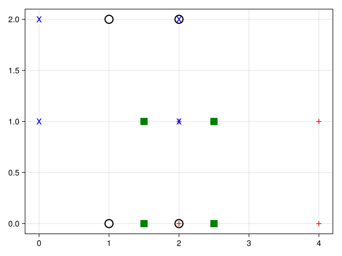

Beyond this there are a few more methods that may be worth implementing when adding a transformation function to the interface:

# Defines the inverse transformation function for a given function.
# Used for example in Axis limits
half(x) = 0.5 * x
Makie.inverse_transform(::typeof(double)) = half

# Defines how bounding boxes are transformed. By default the transformed corners
# are used to build a new bounding box.
Makie.apply_transform(f::typeof(double), r::Rect3) = Rect3(f(origin(r)), f(widths(r)))

# Defines the (1D) limits of an empty Axis using the transform function as the
# xscale or yscale.
Makie.defaultlimits(::typeof(double)) = (0.0, 10.0)

# Defines the range of values that are valid for a given transform function in
# an Axis.
Makie.defined_interval(::typeof(double)) = Makie.OpenInterval(-Inf, Inf)

# Defines how a direction vector at specific position gets transformed. By default
# this transforms two points separated by `delta * direction` to calculate a new
# post-transform direction. The result is normalized.
# Used in `streamplot` and `contour` labels to rotate arrow markers and text
function Makie.apply_transform_to_direction(f::typeof(double), position::VecTypes, direction::VecTypes, delta)
    return direction
end

As an alternative to inverse_transform, defaultlimits and defined_interval a transform function can also be wrapped in a ReversibleScale. This allows bundling the inverse, limits and interval with the transform function.

Makie.ReversibleScale Type

ReversibleScale

Custom scale struct, taking a forward and inverse arbitrary scale function.

Fields

• forward::Function: forward transformation (e.g. log10)

• inverse::Function: inverse transformation (e.g. exp10 for log10 such that inverse ∘ forward ≡ identity)

• limits::Tuple{Float32, Float32}: default limits (optional, defaults to (0, 10))

• interval::IntervalSets.AbstractInterval: valid limits interval (optional, defaults to (-Inf32, Inf32))

• name::Symbol

source