Getting started

Welcome to Makie, the data visualization ecosystem for the Julia language!

This tutorial will show you how to get set up and create plots like this:

Requirements

You only need an internet connection and a reasonably recent Julia installation. If you don't have Julia installed, yet, follow the directions at julialang.org/downloads/.

Makie is available for Windows, Mac and Linux.

Installation

We will be using the CairoMakie package in this tutorial.

Info

Makie offers multiple backend packages that each have different strengths. CairoMakie is good at static 2D graphics and it should run on most computers as it uses only the CPU and does not need a GPU.

First, create a new folder somewhere on your system and call it makie_tutorial. We are going to use that folder to install CairoMakie and to save plots.

Now, start Julia, for example by executing the command julia in a terminal.

In the Julia REPL (the Read-Eval-Print-Loop which is what Julia's command line interface is called), change the active working directory to the makie_tutorial folder by executing this command, but be sure to replace the path with the location where you created the makie_tutorial folder:

cd("path/to/the/folder/makie_tutorial")

Now, make the Pkg package manager library available

using Pkg

Next, activate the current directory, also called "." (this means our makie_tutorial folder), as a Pkg environment:

Pkg.activate(".")

Now, we can install CairoMakie and all its dependencies by running:

Pkg.add("CairoMakie")

This command will probably take a while to finish. You will need an internet connection so all the necessary files can be downloaded.

After this process has completed, you should find a Project.toml and a Manifest.toml file in the makie_tutorial folder. Those files describe the new environment, the downloaded packages are stored somewhere else, in a central, shared location.

If everything has worked, you should be able to load CairoMakie now:

using CairoMakie

Congratulations, now we can start plotting!

Plotting

Run these two lines to make the "data" for our first plot available in your Julia session. It represents some imaginary measurements made over the span of two seconds.

seconds = 0:0.1:2
measurements = [8.2, 8.4, 6.3, 9.5, 9.1, 10.5, 8.6, 8.2, 10.5, 8.5, 7.2,
        8.8, 9.7, 10.8, 12.5, 11.6, 12.1, 12.1, 15.1, 14.7, 13.1]

Let's have a first look at this data as a line plot. Line plots are created with the lines function in Makie.

lines(seconds, measurements)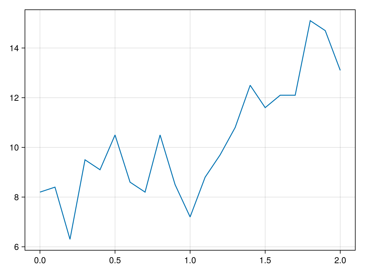

Info

Returning lines(seconds, measurements) in the REPL should show you the plot in some form. Which form it is depends on the context in which you have your Julia REPL running.

If you are in an IDE like VSCode with the Julia extension installed, the plot pane might have opened. If no other display is found, your OS's image viewing application or a browser should show the image.

Let's try another plot function, to show each data point as a separate marker. The right function for that is scatter.

scatter(seconds, measurements)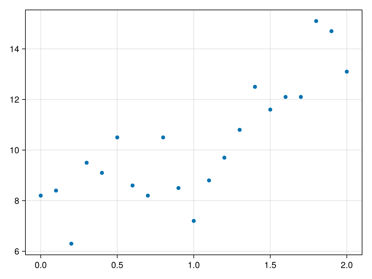

Our goal is to show the measurement data together with a line representing an exponential fit. Let us pretend that the function we have "fit" is f(x) = exp(x) + 7. We can plot it as a line like this:

lines(seconds, exp.(seconds) .+ 7)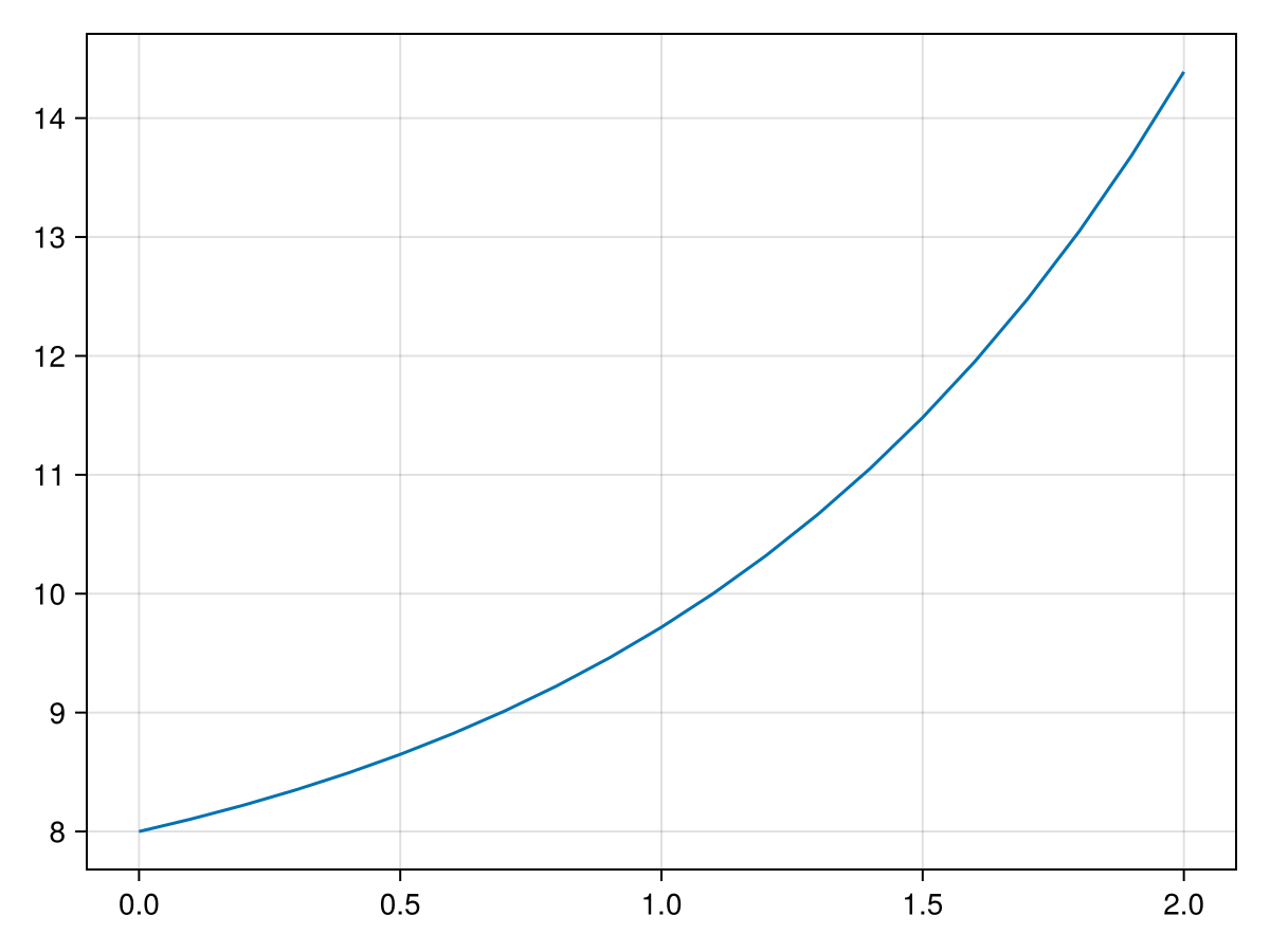

Now, we'd like to have the scatter and lines plots layered on top of each other.

You can plot into an existing axis with plotting functions that end with a !:

scatter(seconds, measurements)
lines!(seconds, exp.(seconds) .+ 7)
current_figure()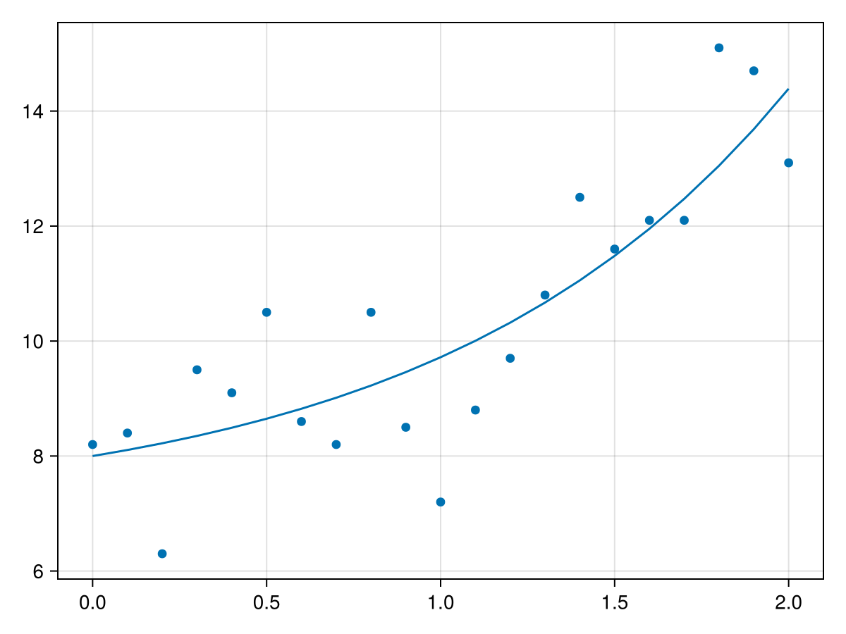

Figure and Axis

So far, we have used two important objects in Makie only implicitly, the Figure and the Axis.

The Figure is the outermost container object. And an Axis is one type of axis object that can contain plots. An Axis can be placed in a Figure and then be plotted into. Let's try the previous plot with this system:

f = Figure()
ax = Axis(f[1, 1])
scatter!(ax, seconds, measurements)
lines!(ax, seconds, exp.(seconds) .+ 7)
f

Both scatter! and lines! now explicitly plot into an Axis which we put into a Figure. Axis(f[1, 1]) means that we put the Axis at the Figure's layout at position row 1, column 1.

We can now give our Axis a title, as well as x and y axis labels:

f = Figure()
ax = Axis(f[1, 1],
    title = "Experimental data and exponential fit",
    xlabel = "Time (seconds)",
    ylabel = "Value",
)
scatter!(ax, seconds, measurements)
lines!(ax, seconds, exp.(seconds) .+ 7)
f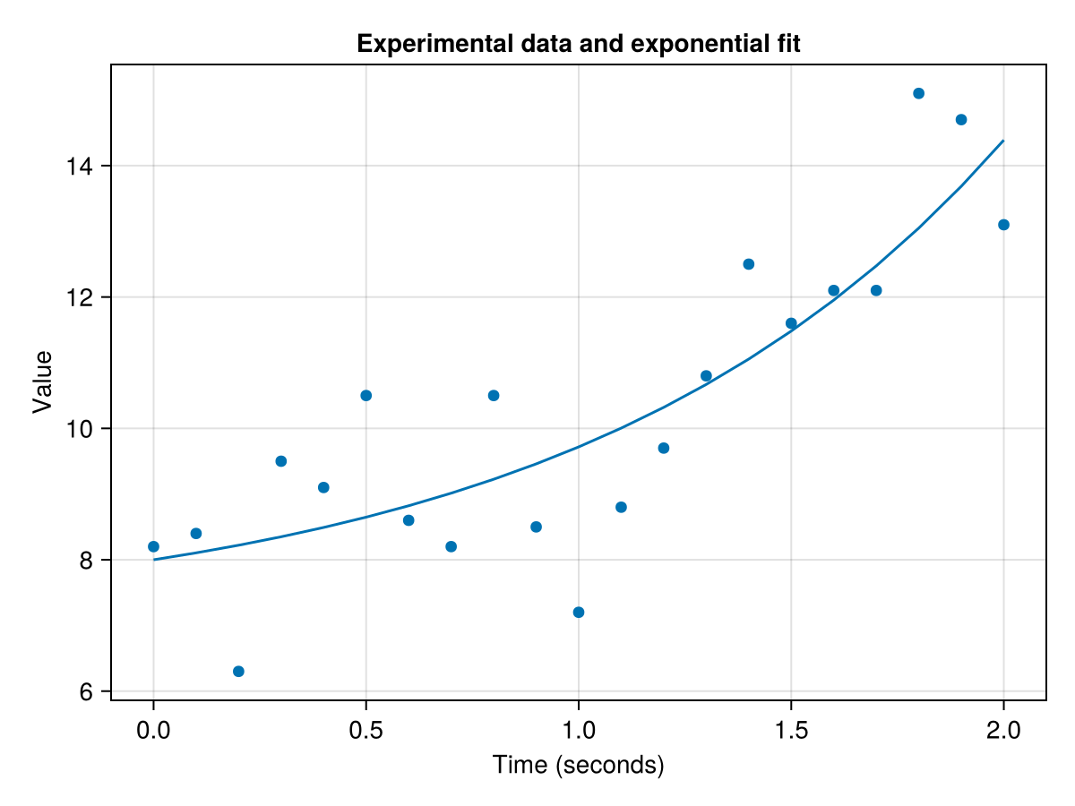

Plot styling

Plotting functions take many different style attributes as keyword arguments. Let's change the color of both plots to a red called :tomato, and the line style to :dash:

f = Figure()
ax = Axis(f[1, 1],
    title = "Experimental data and exponential fit",
    xlabel = "Time (seconds)",
    ylabel = "Value",
)
scatter!(ax, seconds, measurements, color = :tomato)
lines!(ax, seconds, exp.(seconds) .+ 7, color = :tomato, linestyle = :dash)
f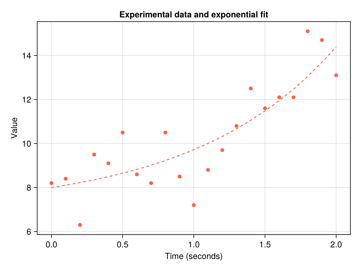

Legend

The last element we're missing is the legend. One way to create a legend is by labelling plots with the label keyword and using the axislegend function:

f = Figure()
ax = Axis(f[1, 1],
    title = "Experimental data and exponential fit",
    xlabel = "Time (seconds)",
    ylabel = "Value",
)
scatter!(
    ax,
    seconds,
    measurements,
    color = :tomato,
    label = "Measurements"
)
lines!(
    ax,
    seconds,
    exp.(seconds) .+ 7,
    color = :tomato,
    linestyle = :dash,
    label = "f(x) = exp(x) + 7",
)
axislegend(position = :rb)
f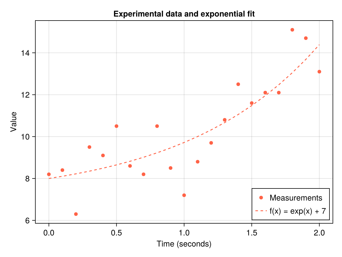

Saving a Figure

Once we are satisfied with our plot, we can save it to a file using the save function. The most common formats are png for images and svg or pdf for vector graphics:

save("first_figure.png", f)
save("first_figure.svg", f)
save("first_figure.pdf", f)

You should now find the three files in your makie_tutorial folder.