surface
Makie.surface Function
surface(x, y, z)
surface(z)
Plots a surface, where (x, y) define a grid whose heights are the entries in z. x and y may be Vectors which define a regular grid, or Matrices which define an irregular grid.
Plot type
The plot type alias for the surface function is Surface.
Examples
Gridded surfaces
By default surface data is placed on a grid matching the size of the input data. The grid can be specified explicitly by passing a Range or Vector of values as the X and Y arguments. The positions/vertices of the surface are then effectively derived as Point.(X, Y', Z). Intervals (e.g 0..1) can be used to specify the start and endpoint only, implying a linear range in between.
using GLMakie
xs = LinRange(0, 10, 100)
ys = LinRange(0, 15, 100)
zs = [cos(x) * sin(y) for x in xs, y in ys]

surface(xs, ys, zs, axis=(type=Axis3,))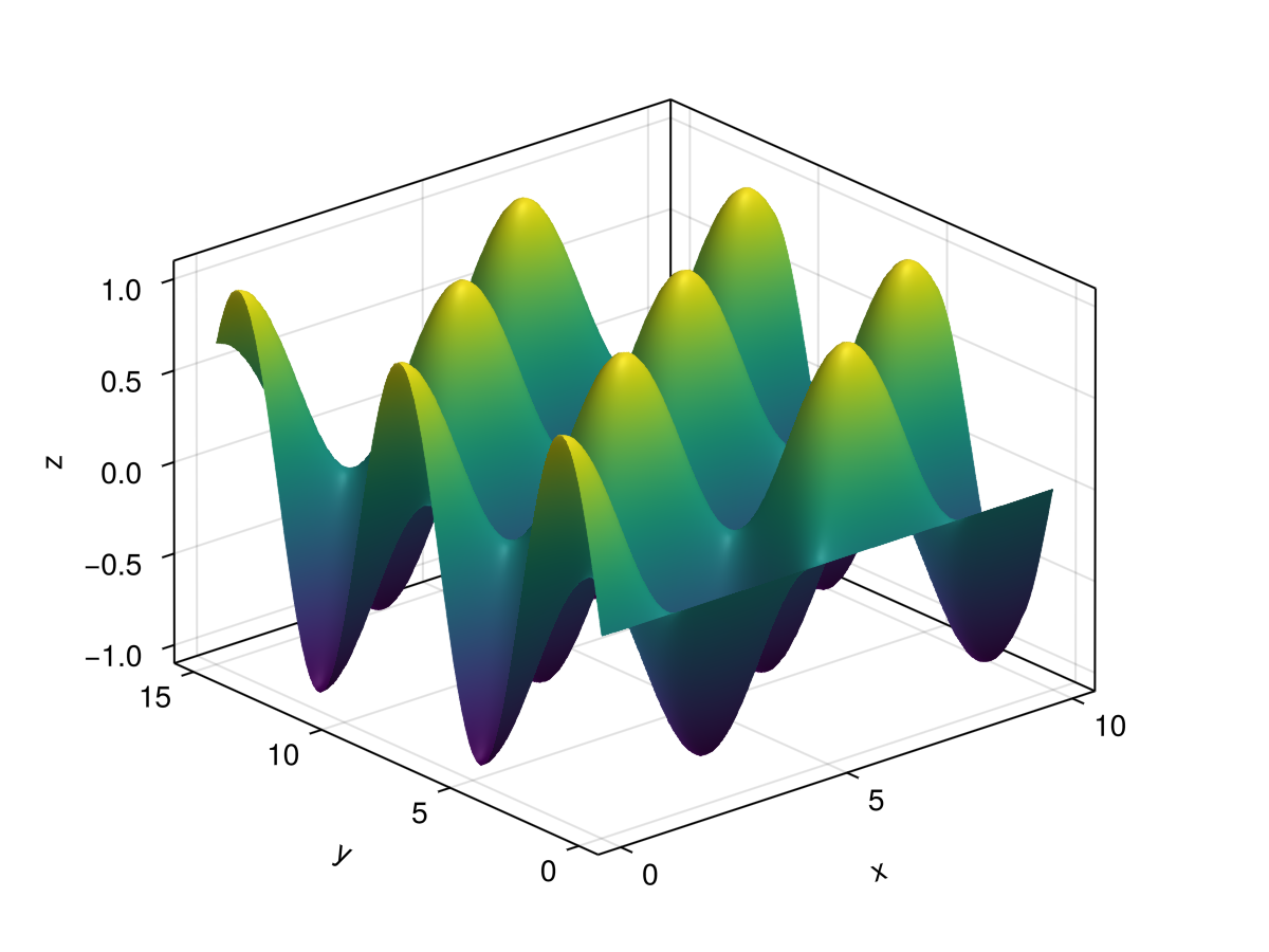
using GLMakie
using DelimitedFiles

volcano = readdlm(Makie.assetpath("volcano.csv"), ',', Float64)

surface(volcano,
    colormap = :darkterrain,
    colorrange = (80, 190),
    axis=(type=Axis3, azimuth = pi/4))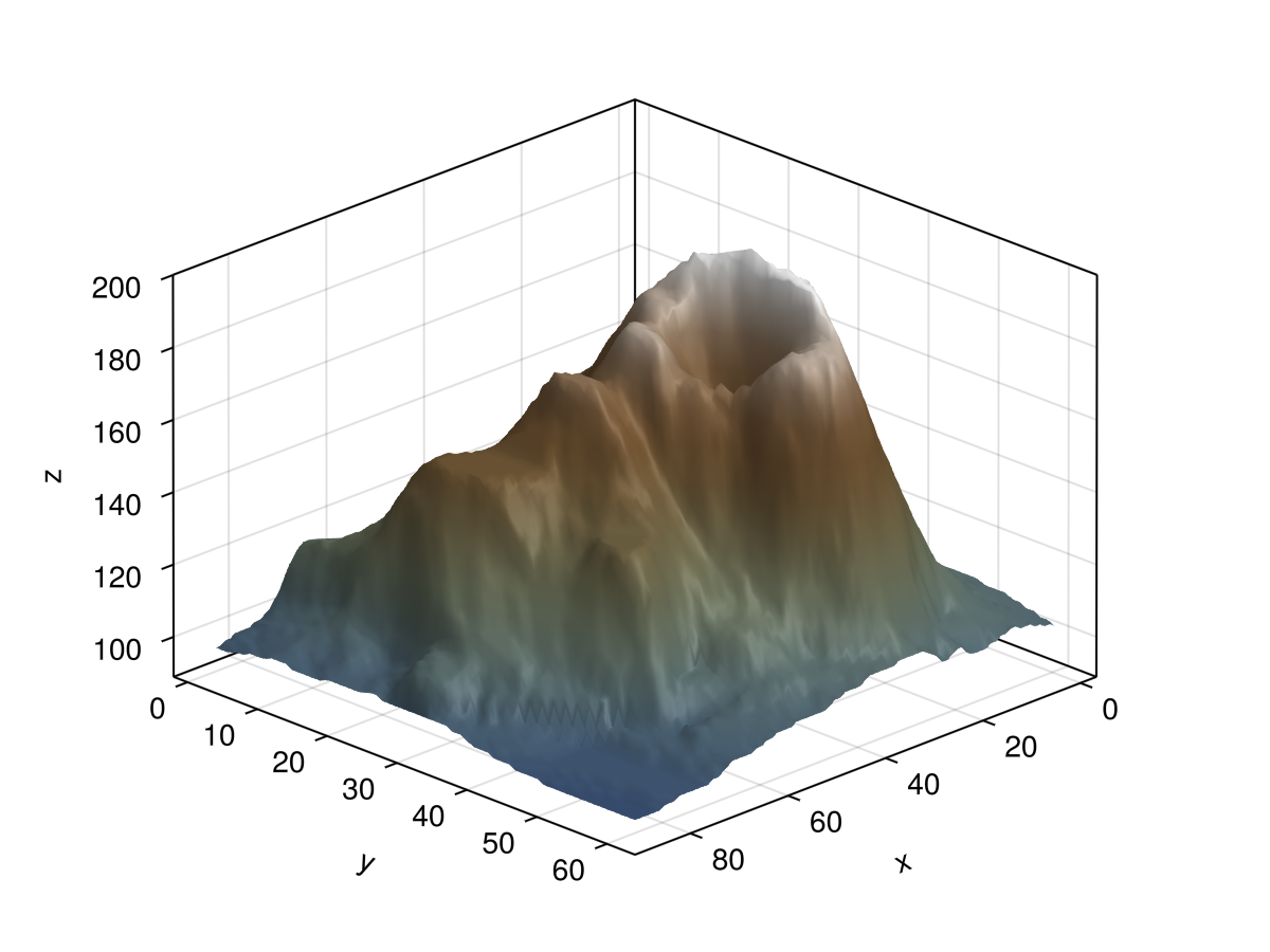
using GLMakie
using SparseArrays
using LinearAlgebra

# This example was provided by Moritz Schauer (@mschauer).

#=
Define the precision matrix (inverse covariance matrix)
for the Gaussian noise matrix.  It approximately coincides
with the Laplacian of the 2d grid or the graph representing
the neighborhood relation of pixels in the picture,
https://en.wikipedia.org/wiki/Laplacian_matrix
=#
function gridlaplacian(m, n)
    S = sparse(0.0I, n*m, n*m)
    linear = LinearIndices((1:m, 1:n))
    for i in 1:m
        for j in 1:n
            for (i2, j2) in ((i + 1, j), (i, j + 1))
                if i2 <= m && j2 <= n
                    S[linear[i, j], linear[i2, j2]] -= 1
                    S[linear[i2, j2], linear[i, j]] -= 1
                    S[linear[i, j], linear[i, j]] += 1
                    S[linear[i2, j2], linear[i2, j2]] += 1
                end
            end
        end
    end
    return S
end

# d is used to denote the size of the data
d = 150

 # Sample centered Gaussian noise with the right correlation by the method
 # based on the Cholesky decomposition of the precision matrix
data = 0.1randn(d,d) + reshape(
        cholesky(gridlaplacian(d,d) + 0.003I) \ randn(d*d),
        d, d
)

surface(data; shading = NoShading, colormap = :deep)
surface(data; shading = NoShading, colormap = :deep)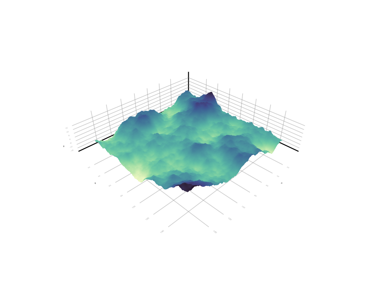
Quad Mesh surface
X and Y values can also be given as a Matrix. In this case the surface positions follow as Point.(X, Y, Z) so the surface is no longer restricted to an XY grid.
using GLMakie
rs = 1:10
thetas = 0:10:360

xs = rs .* cosd.(thetas')
ys = rs .* sind.(thetas')
zs = sin.(rs) .* cosd.(thetas')

surface(xs, ys, zs)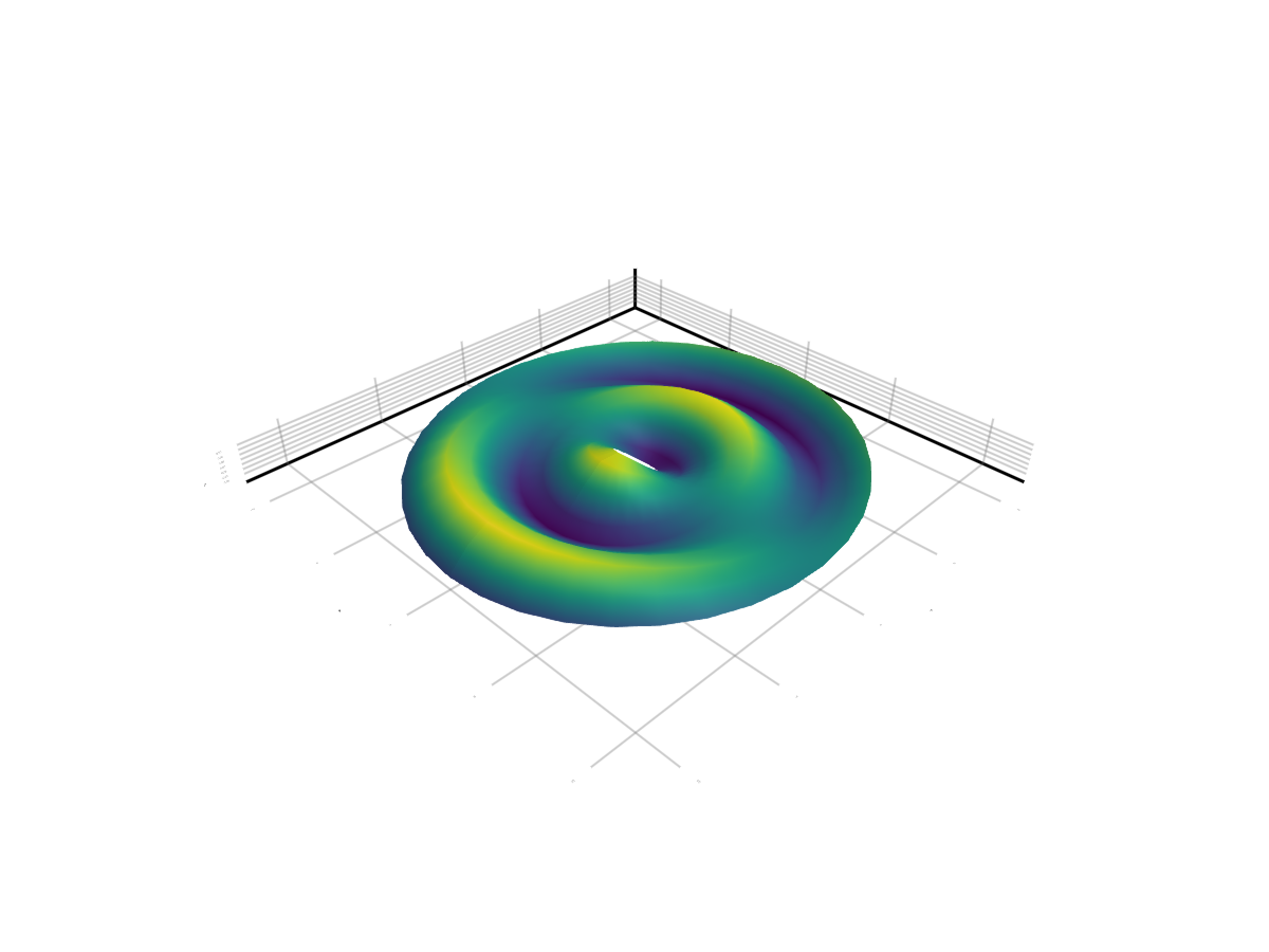
NaN Handling
If a vertex of the surface is NaN, meaning that either X, Y or Z contribute NaN to it, all connected faces can not be drawn. Thus the surface will have a hole around a NaN vertex. If just a color is NaN it will be drawn with nan_color.
using GLMakie
xs = ys = vcat(1:9, NaN, 11:30)
zs = [2 * sin(x+y) for x in range(-3, 3, length=30), y in range(-3, 3, length=30)]
zs_nan = copy(zs)
zs_nan[25, 25] = NaN

f = Figure(size = (600, 300))
surface(f[1, 1], xs, ys, zs_nan, axis = (show_axis = false,))
surface(f[1, 2], 1:30, 1:30, zs, color = zs_nan, nan_color = :red, axis = (show_axis = false,))
f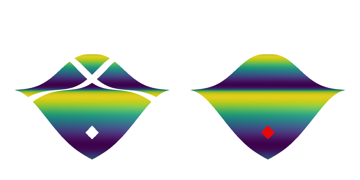
2D Surface
A surface plot can act as an off-grid version of heatmap or image in 2D. For this it is recommended to pass data through color instead of the Z argument to avoid the plot interfering with others based on its Z values.
using GLMakie
rs = 1:10
thetas = 0:10:360

xs = rs .* cosd.(thetas')
ys = rs .* sind.(thetas')
zs = sin.(rs) .* cosd.(thetas')

surface(xs, ys, zeros(size(zs)), color = zs, shading = NoShading)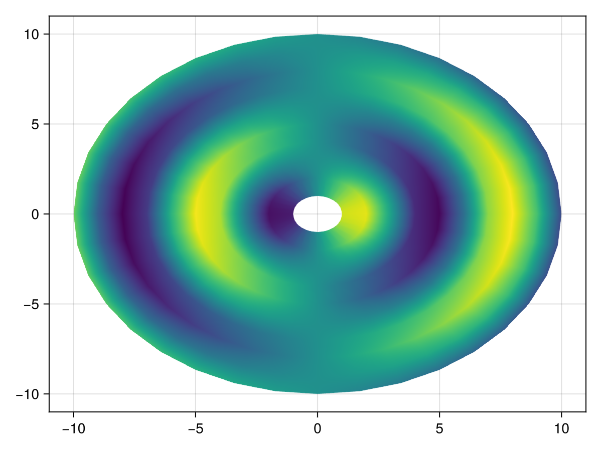
Attributes
alpha
Defaults to 1.0
The alpha value of the colormap or color attribute. Multiple alphas like in plot(alpha=0.2, color=(:red, 0.5)), will get multiplied.
backlight
Defaults to 0.0
Sets a weight for secondary light calculation with inverted normals.
clip_planes
Defaults to @inherit clip_planes automatic
Clip planes offer a way to do clipping in 3D space. You can set a Vector of up to 8 Plane3f planes here, behind which plots will be clipped (i.e. become invisible). By default clip planes are inherited from the parent plot or scene. You can remove parent clip_planes by passing Plane3f[].
color
Defaults to nothing
Can be set to an Matrix{<: Union{Number, Colorant}} to color surface independent of the z component. If color=nothing, it defaults to color=z. Can also be a Makie.AbstractPattern.
colormap
Defaults to @inherit colormap :viridis
Sets the colormap that is sampled for numeric colors. PlotUtils.cgrad(...), Makie.Reverse(any_colormap) can be used as well, or any symbol from ColorBrewer or PlotUtils. To see all available color gradients, you can call Makie.available_gradients().
colorrange
Defaults to automatic
The values representing the start and end points of colormap.
colorscale
Defaults to identity
The color transform function. Can be any function, but only works well together with Colorbar for identity, log, log2, log10, sqrt, logit, Makie.pseudolog10, Makie.Symlog10, Makie.AsinhScale, Makie.SinhScale, Makie.LogScale, Makie.LuptonAsinhScale, and Makie.PowerScale.
depth_shift
Defaults to 0.0
Adjusts the depth value of a plot after all other transformations, i.e. in clip space, where -1 <= depth <= 1. This only applies to GLMakie and WGLMakie and can be used to adjust render order (like a tunable overdraw).
diffuse
Defaults to 1.0
Sets how strongly the red, green and blue channel react to diffuse (scattered) light.
fxaa
Defaults to true
Adjusts whether the plot is rendered with fxaa (fast approximate anti-aliasing, GLMakie only). Note that some plots implement a better native anti-aliasing solution (scatter, text, lines). For them fxaa = true generally lowers quality. Plots that show smoothly interpolated data (e.g. image, surface) may also degrade in quality as fxaa = true can cause blurring.
highclip
Defaults to automatic
The color for any value above the colorrange.
inspectable
Defaults to @inherit inspectable
Sets whether this plot should be seen by DataInspector. The default depends on the theme of the parent scene.
inspector_clear
Defaults to automatic
Sets a callback function (inspector, plot) -> ... for cleaning up custom indicators in DataInspector.
inspector_hover
Defaults to automatic
Sets a callback function (inspector, plot, index) -> ... which replaces the default show_data methods.
inspector_label
Defaults to automatic
Sets a callback function (plot, index, position) -> string which replaces the default label generated by DataInspector.
interpolate
Defaults to true
[(W)GLMakie only] Specifies whether the surface matrix gets sampled with interpolation.
invert_normals
Defaults to false
Inverts the normals generated for the surface. This can be useful to illuminate the other side of the surface.
lowclip
Defaults to automatic
The color for any value below the colorrange.
matcap
Defaults to nothing
Applies a "material capture" texture to the generated mesh. A matcap encodes lighting and color data of a material on a circular texture which is sampled based on normal vectors.
material
Defaults to nothing
RPRMakie only attribute to set complex RadeonProRender materials. Warning, how to set an RPR material may change and other backends will ignore this attribute
model
Defaults to automatic
Sets a model matrix for the plot. This overrides adjustments made with translate!, rotate! and scale!.
nan_color
Defaults to :transparent
The color for NaN values.
overdraw
Defaults to false
Controls if the plot will draw over other plots. This specifically means ignoring depth checks in GL backends
shading
Defaults to true
Controls if the plot object is shaded by the parent scenes lights or not. The lighting algorithm used is controlled by the scenes shading attribute.
shininess
Defaults to 32.0
Sets how sharp the reflection is.
space
Defaults to :data
Sets the transformation space for box encompassing the plot. See Makie.spaces() for possible inputs.
specular
Defaults to 0.2
Sets how strongly the object reflects light in the red, green and blue channels.
ssao
Defaults to false
Adjusts whether the plot is rendered with ssao (screen space ambient occlusion). Note that this only makes sense in 3D plots and is only applicable with fxaa = true.
transformation
Defaults to :automatic
Controls the inheritance or directly sets the transformations of a plot. Transformations include the transform function and model matrix as generated by translate!(...), scale!(...) and rotate!(...). They can be set directly by passing a Transformation() object or inherited from the parent plot or scene. Inheritance options include:
:automatic: Inherit transformations if the parent and childspaceis compatible:inherit: Inherit transformations:inherit_model: Inherit only model transformations:inherit_transform_func: Inherit only the transform function:nothing: Inherit neither, fully disconnecting the child's transformations from the parent
Another option is to pass arguments to the transform!() function which then get applied to the plot. For example transformation = (:xz, 1.0) which rotates the xy plane to the xz plane and translates by 1.0. For this inheritance defaults to :automatic but can also be set through e.g. (:nothing, (:xz, 1.0)).
transparency
Defaults to false
Adjusts how the plot deals with transparency. In GLMakie transparency = true results in using Order Independent Transparency.
uv_transform
Defaults to automatic
Sets a transform for uv coordinates, which controls how a texture is mapped to a surface. The attribute can be I, scale::VecTypes{2}, (translation::VecTypes{2}, scale::VecTypes{2}), any of :rotr90, :rotl90, :rot180, :swap_xy/:transpose, :flip_x, :flip_y, :flip_xy, or most generally a Makie.Mat{2, 3, Float32} or Makie.Mat3f as returned by Makie.uv_transform(). They can also be changed by passing a tuple (op3, op2, op1).
visible
Defaults to true
Controls whether the plot gets rendered or not.