Plot methods
Makie offers a simple but powerful set of methods for each plotting function, which allow you to easily create and manipulate the most common aspects of a figure.
Each plot object like Scatter has two plotting functions associated to it, a non-mutating version (scatter) and a mutating version (scatter!). These functions have different methods that behave slightly differently depending on the first argument.
Here's a short list before we show each version in more detail. We use Scatter as our example, but the principles apply to every plot type.
Non-Mutating
The non-mutating methods create and return something in addition to the plot object, either a figure with an axis in default position, or an axis at a given GridPosition or GridSubposition.
scatter(args...; kwargs...) -> ::FigureAxisPlot
scatter(gridposition, args...; kwargs...) -> ::AxisPlot
FigureAxisPlot is just a collection of the new figure, axis and plot. For convenience it has the same display overload as Figure, so that scatter(args...) displays a plot without further work. It can be destructured at assignment like fig, ax, plotobj = scatter(args...).
AxisPlot is a collection of a new axis and plot. It has no special display overload but can also be destructured like ax, plotobj = scatter(gridposition, args...).
Special Keyword Arguments
Methods that create an AxisPlot accept a special-cased axis keyword, where you can pass a dict-like object containing keyword arguments that should be passed to the created axis. Methods that create a FigureAxisPlot additionally accept a special cased figure keyword, where you can pass a dict-like object containing keyword arguments that should be passed to the created figure.
All other keyword arguments are passed as attributes to the plotting function.
Here are two examples with the scatter function (take care to create single-argument NamedTuples correctly, for example with a trailing comma):
using CairoMakie
# FigureAxisPlot takes figure and axis keywords
fig, ax, p = lines(cumsum(randn(1000)),
    figure = (size = (1000, 600),),
    axis = (ylabel = "Temperature",),
    color = :red)

# AxisPlot takes axis keyword
lines(fig[2, 1], cumsum(randn(1000)),
    axis = (xlabel = "Time (sec)", ylabel = "Stock Value"),
    color = :blue)

fig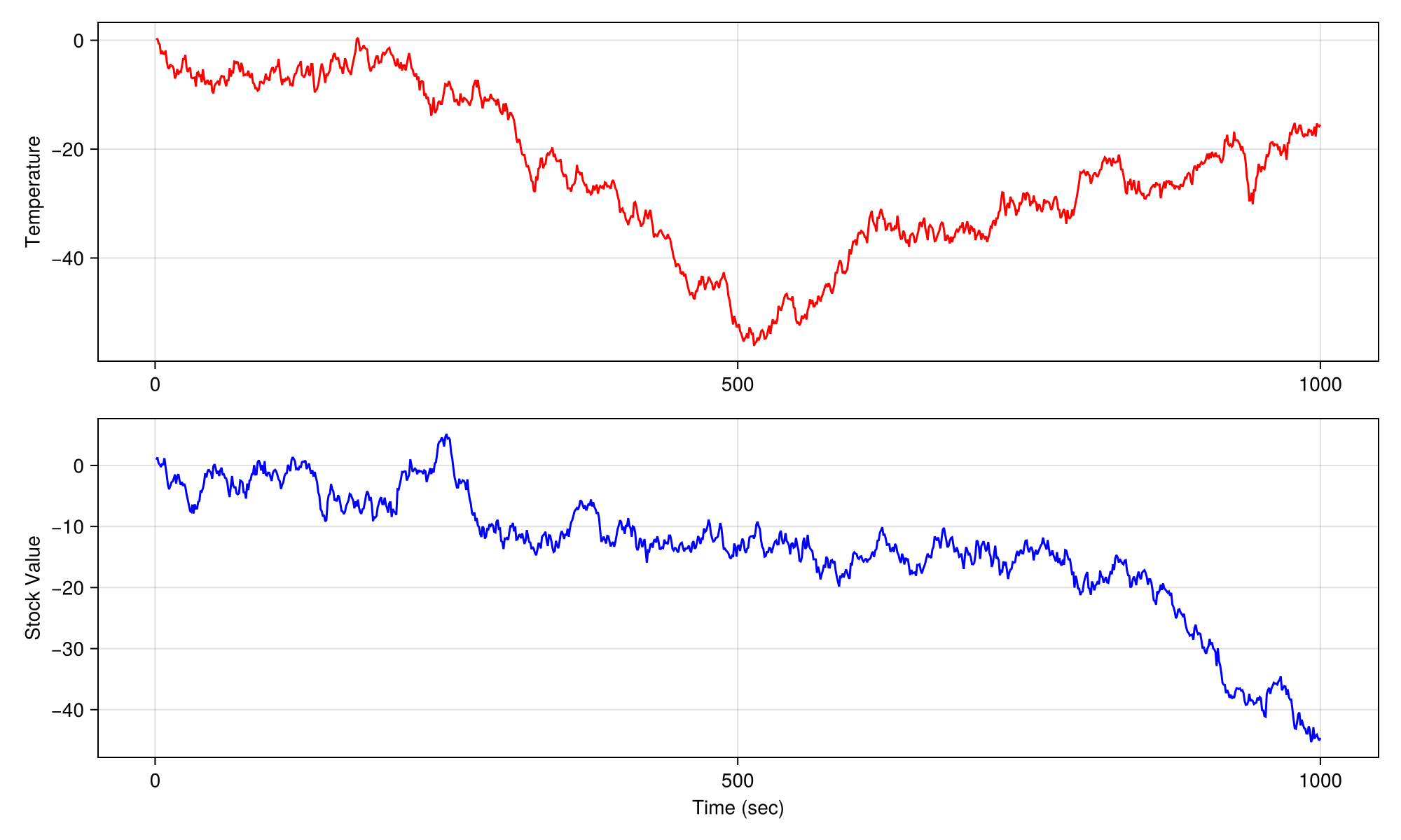
Mutating
The mutating methods always just return a plot object. If no figure is passed, the current_figure() is used, if no axis or scene is given, the current_axis() is used.
scatter!(args...; kwargs...) -> ::Scatter
scatter!(figure, args...; kwargs...) -> ::Scatter
scatter!(gridposition, args...; kwargs...) -> ::Scatter
scatter!(axis, args...; kwargs...) -> ::Scatter
scatter!(scene, args...; kwargs...) -> ::Scatter
GridPositions
In the background, each Figure has a GridLayout from GridLayoutBase.jl, which takes care of layouting plot elements nicely. For convenience, you can index into a figure multiple times to refer to nested grid positions, which makes it easy to quickly assemble complex layouts.
For example, fig[1, 2] creates a GridPosition referring to row 1 and column 2, while fig[1, 2][3, 1:2] creates a GridSubposition that refers to row 3 and columns 1 to 2 in a nested GridLayout which is located at row 1 and column 2. The link to the Figure is in the parent field of the top layout.
With Non-Mutating Plotting Functions
Using the non-mutating plotting functions with GridPositions creates new axes at the given locations. If a GridLayout along the nesting levels doesn't exist, yet, it is created automatically for convenience.
using CairoMakie
fig = Figure()

# first row, first column
scatter(fig[1, 1], 1.0..10, sin)

# first row, second column
lines(fig[1, 2], 1.0..10, sin)

# first row, third column, then nested first row, first column
lines(fig[1, 3][1, 1], cumsum(randn(1000)), color = :blue)

# first row, third column, then nested second row, first column
lines(fig[1, 3][2, 1], cumsum(randn(1000)), color = :red)

# second row, first to third column
ax, hm = heatmap(fig[2, 1:3], randn(30, 10))

# across all rows, new column after the last one
fig[:, end+1] = Colorbar(fig, hm)

fig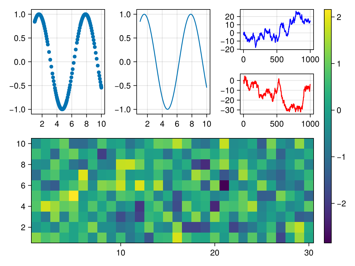
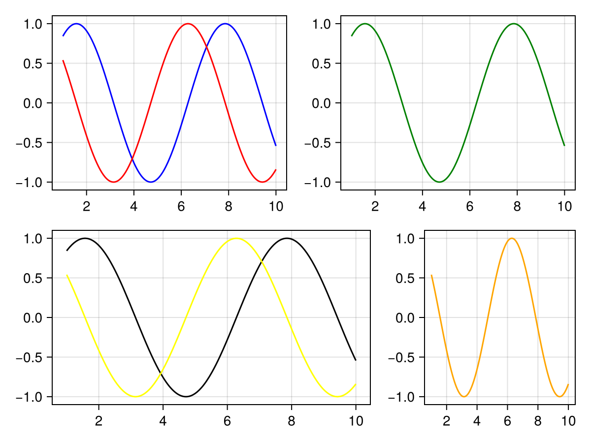
With Mutating Plotting Functions
Mutating plotting functions work a bit differently with GridPositions. First, it is checked if one - and only one - axis exists already at the given position. If that's the case, that axis is plotted into. If it's not the case, the function will error.
using CairoMakie
fig = Figure()

lines(fig[1, 1], 1.0..10, sin, color = :blue)
# this works because the previous command created an axis at fig[1, 1]
lines!(fig[1, 1], 1.0..10, cos, color = :red)

# the following line wouldn't work yet because no axis exists at fig[1, 2]
# lines!(fig[1, 2], 1.0..10, sin, color = :green)

fig[1, 2] = Axis(fig)
# now it works
lines!(fig[1, 2], 1.0..10, sin, color = :green)

# also works with nested grids
fig[2, 1:2][1, 3] = Axis(fig)
lines!(fig[2, 1:2][1, 3], 1.0..10, cos, color = :orange)

# but often it's more convenient to save an axis to reuse it
ax, _ = lines(fig[2, 1:2][1, 1:2], 1.0..10, sin, color = :black)
lines!(ax, 1.0..10, cos, color = :yellow)

fig