tricontourf

julia

tricontourf(triangles::Triangulation, zs; kwargs...)
tricontourf(xs, ys, zs; kwargs...)

Plots a filled tricontour of the height information in zs at the horizontal positions xs and vertical positions ys. A Triangulation from DelaunayTriangulation.jl can also be provided instead of xs and ys for specifying the triangles, otherwise an unconstrained triangulation of xs and ys is computed.

Plot type

The plot type alias for the tricontourf function is Tricontourf.

source

Examples

julia

using CairoMakie
using Random
Random.seed!(1234)

x = randn(50)
y = randn(50)
z = -sqrt.(x .^ 2 .+ y .^ 2) .+ 0.1 .* randn.()

f, ax, tr = tricontourf(x, y, z)
scatter!(x, y, color = z, strokewidth = 1, strokecolor = :black)
Colorbar(f[1, 2], tr)
f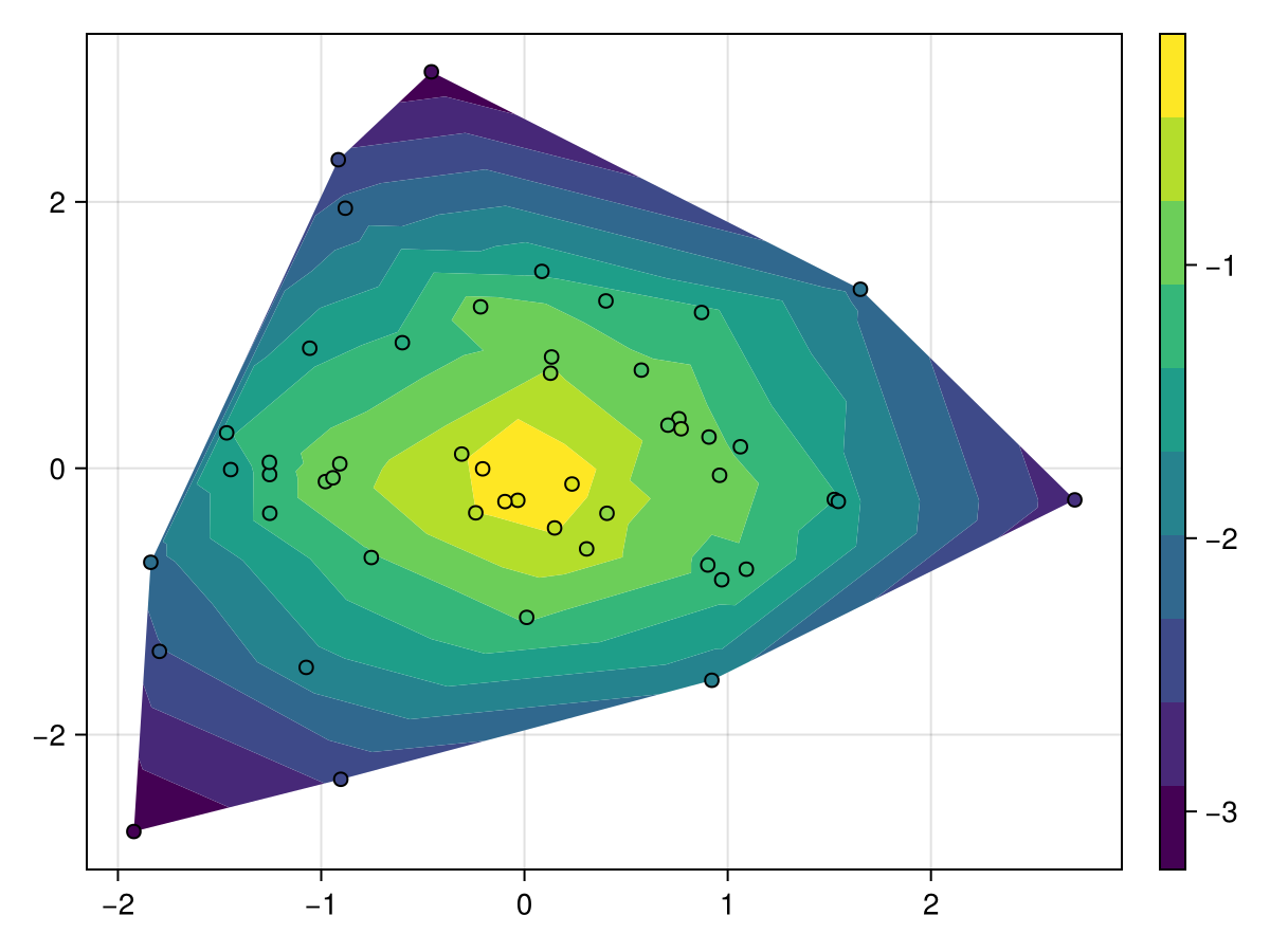

julia

using CairoMakie
using Random
Random.seed!(1234)

x = randn(200)
y = randn(200)
z = x .* y

f, ax, tr = tricontourf(x, y, z, colormap = :batlow)
scatter!(x, y, color = z, colormap = :batlow, strokewidth = 1, strokecolor = :black)
Colorbar(f[1, 2], tr)
f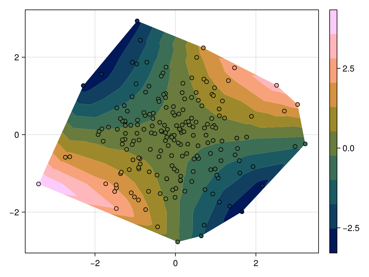

Triangulation modes

Manual triangulations can be passed as a 3xN matrix of integers, where each column of three integers specifies the indices of the corners of one triangle in the vector of points.

julia

using CairoMakie
using Random
Random.seed!(123)

n = 20
angles = range(0, 2pi, length = n+1)[1:end-1]
x = [cos.(angles); 2 .* cos.(angles .+ pi/n)]
y = [sin.(angles); 2 .* sin.(angles .+ pi/n)]
z = (x .- 0.5).^2 + (y .- 0.5).^2 .+ 0.5.*randn.()

triangulation_inner = reduce(hcat, map(i -> [0, 1, n] .+ i, 1:n))
triangulation_outer = reduce(hcat, map(i -> [n-1, n, 0] .+ i, 1:n))
triangulation = hcat(triangulation_inner, triangulation_outer)

f, ax, _ = tricontourf(x, y, z, triangulation = triangulation,
    axis = (; aspect = 1, title = "Manual triangulation"))
scatter!(x, y, color = z, strokewidth = 1, strokecolor = :black)

tricontourf(f[1, 2], x, y, z, triangulation = Makie.DelaunayTriangulation(),
    axis = (; aspect = 1, title = "Delaunay triangulation"))
scatter!(x, y, color = z, strokewidth = 1, strokecolor = :black)

f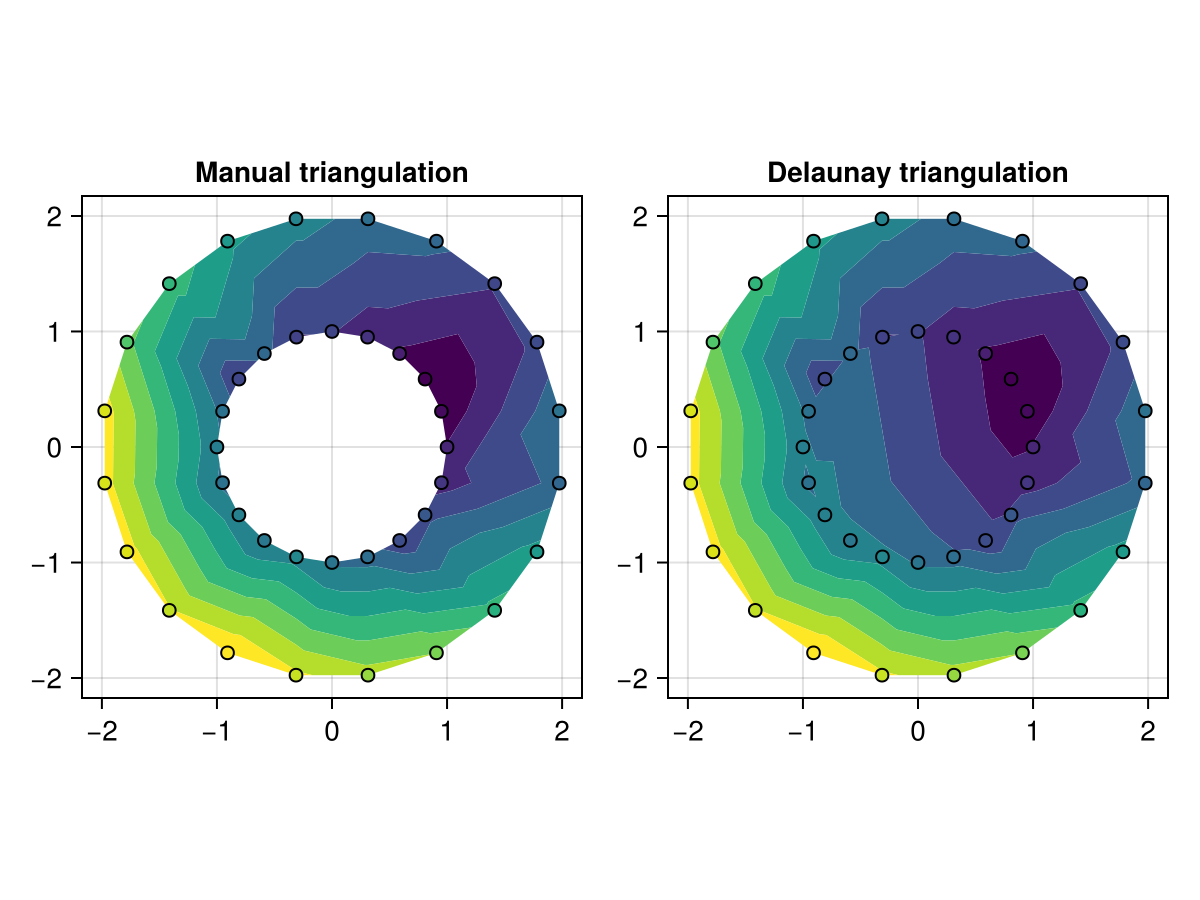

By default, tricontourf performs unconstrained triangulations. Greater control over the triangulation, such as allowing for enforced boundaries, can be achieved by using DelaunayTriangulation.jl and passing the resulting triangulation as the first argument of tricontourf. For example, the above annulus can also be plotted as follows:

julia

using CairoMakie
using DelaunayTriangulation
using Random

Random.seed!(123)

n = 20
angles = range(0, 2pi, length = n+1)[1:end-1]
x = [cos.(angles); 2 .* cos.(angles .+ pi/n)]
y = [sin.(angles); 2 .* sin.(angles .+ pi/n)]
z = (x .- 0.5).^2 + (y .- 0.5).^2 .+ 0.5.*randn.()

inner = [n:-1:1; n] # clockwise inner
outer = [(n+1):(2n); n+1] # counter-clockwise outer
boundary_nodes = [[outer], [inner]]
points = [x'; y']
tri = triangulate(points; boundary_nodes = boundary_nodes)
f, ax, _ = tricontourf(tri, z;
    axis = (; aspect = 1, title = "Constrained triangulation\nvia DelaunayTriangulation.jl"))
scatter!(x, y, color = z, strokewidth = 1, strokecolor = :black)
f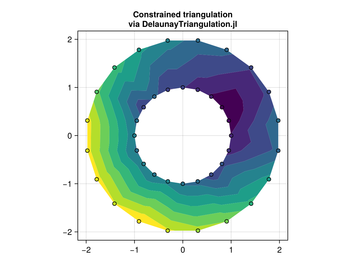

Boundary nodes make it possible to support more complicated regions, possibly with holes, than is possible by only providing points themselves.

julia

using CairoMakie
using DelaunayTriangulation

## Start by defining the boundaries, and then convert to the appropriate interface
curve_1 = [
    [(0.0, 0.0), (5.0, 0.0), (10.0, 0.0), (15.0, 0.0), (20.0, 0.0), (25.0, 0.0)],
    [(25.0, 0.0), (25.0, 5.0), (25.0, 10.0), (25.0, 15.0), (25.0, 20.0), (25.0, 25.0)],
    [(25.0, 25.0), (20.0, 25.0), (15.0, 25.0), (10.0, 25.0), (5.0, 25.0), (0.0, 25.0)],
    [(0.0, 25.0), (0.0, 20.0), (0.0, 15.0), (0.0, 10.0), (0.0, 5.0), (0.0, 0.0)]
] # outer-most boundary: counter-clockwise
curve_2 = [
    [(4.0, 6.0), (4.0, 14.0), (4.0, 20.0), (18.0, 20.0), (20.0, 20.0)],
    [(20.0, 20.0), (20.0, 16.0), (20.0, 12.0), (20.0, 8.0), (20.0, 4.0)],
    [(20.0, 4.0), (16.0, 4.0), (12.0, 4.0), (8.0, 4.0), (4.0, 4.0), (4.0, 6.0)]
] # inner boundary: clockwise
curve_3 = [
    [(12.906, 10.912), (16.0, 12.0), (16.16, 14.46), (16.29, 17.06),
    (13.13, 16.86), (8.92, 16.4), (8.8, 10.9), (12.906, 10.912)]
] # this is inside curve_2, so it's counter-clockwise
curves = [curve_1, curve_2, curve_3]
points = [
    (3.0, 23.0), (9.0, 24.0), (9.2, 22.0), (14.8, 22.8), (16.0, 22.0),
    (23.0, 23.0), (22.6, 19.0), (23.8, 17.8), (22.0, 14.0), (22.0, 11.0),
    (24.0, 6.0), (23.0, 2.0), (19.0, 1.0), (16.0, 3.0), (10.0, 1.0), (11.0, 3.0),
    (6.0, 2.0), (6.2, 3.0), (2.0, 3.0), (2.6, 6.2), (2.0, 8.0), (2.0, 11.0),
    (5.0, 12.0), (2.0, 17.0), (3.0, 19.0), (6.0, 18.0), (6.5, 14.5),
    (13.0, 19.0), (13.0, 12.0), (16.0, 8.0), (9.8, 8.0), (7.5, 6.0),
    (12.0, 13.0), (19.0, 15.0)
]
boundary_nodes, points = convert_boundary_points_to_indices(curves; existing_points=points)
edges = Set(((1, 19), (19, 12), (46, 4), (45, 12)))

## Extract the x, y
tri = triangulate(points; boundary_nodes = boundary_nodes, segments = edges)
z = [(x - 1) * (y + 1) for (x, y) in DelaunayTriangulation.each_point(tri)] # note that each_point preserves the index order
f, ax, _ = tricontourf(tri, z, levels = 30; axis = (; aspect = 1))
f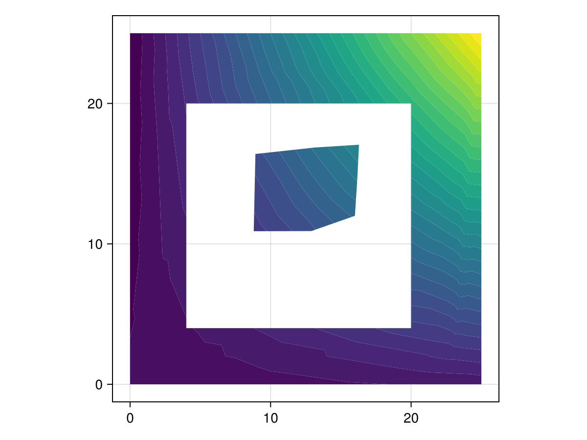

julia

using CairoMakie
using DelaunayTriangulation

using Random
Random.seed!(1234)

θ = [LinRange(0, 2π * (1 - 1/19), 20); 0]
xy = Vector{Vector{Vector{NTuple{2,Float64}}}}()
cx = [0.0, 3.0]
for i in 1:2
    push!(xy, [[(cx[i] + cos(θ), sin(θ)) for θ in θ]])
    push!(xy, [[(cx[i] + 0.5cos(θ), 0.5sin(θ)) for θ in reverse(θ)]])
end
boundary_nodes, points = convert_boundary_points_to_indices(xy)
tri = triangulate(points; boundary_nodes=boundary_nodes)
z = [(x - 3/2)^2 + y^2 for (x, y) in DelaunayTriangulation.each_point(tri)] # note that each_point preserves the index order

f, ax, tr = tricontourf(tri, z, colormap = :matter)
f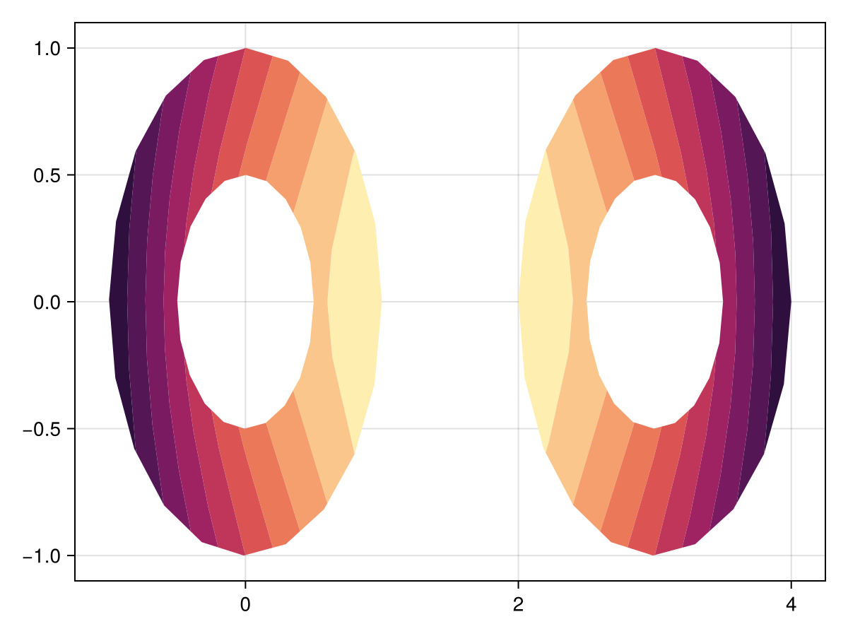

Relative mode

Sometimes it's beneficial to drop one part of the range of values, usually towards the outer boundary. Rather than specifying the levels to include manually, you can set the mode attribute to :relative and specify the levels from 0 to 1, relative to the current minimum and maximum value.

julia

using CairoMakie
using Random
Random.seed!(1234)

x = randn(50)
y = randn(50)
z = -sqrt.(x .^ 2 .+ y .^ 2) .+ 0.1 .* randn.()

f, ax, tr = tricontourf(x, y, z, mode = :relative, levels = 0.2:0.1:1)
scatter!(x, y, color = z, strokewidth = 1, strokecolor = :black)
Colorbar(f[1, 2], tr)
f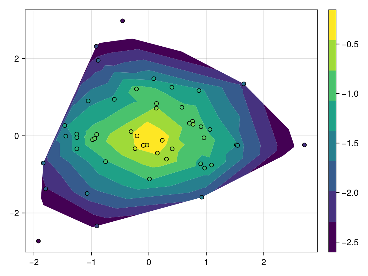

Attributes

clip_planes

Defaults to automatic

Clip planes offer a way to do clipping in 3D space. You can set a Vector of up to 8 Plane3f planes here, behind which plots will be clipped (i.e. become invisible). By default clip planes are inherited from the parent plot or scene. You can remove parent clip_planes by passing Plane3f[].

colormap

Defaults to @inherit colormap

Sets the colormap from which the band colors are sampled.

colorscale

Defaults to identity

Color transform function

depth_shift

Defaults to 0.0

adjusts the depth value of a plot after all other transformations, i.e. in clip space, where 0 <= depth <= 1. This only applies to GLMakie and WGLMakie and can be used to adjust render order (like a tunable overdraw).

edges

Defaults to nothing

No docs available.

extendhigh

Defaults to nothing

This sets the color of an optional additional band from the highest value of levels to maximum(zs). If it's :auto, the high end of the colormap is picked and the remaining colors are shifted accordingly. If it's any color representation, this color is used. If it's nothing, no band is added.

extendlow

Defaults to nothing

This sets the color of an optional additional band from minimum(zs) to the lowest value in levels. If it's :auto, the lower end of the colormap is picked and the remaining colors are shifted accordingly. If it's any color representation, this color is used. If it's nothing, no band is added.

fxaa

Defaults to true

adjusts whether the plot is rendered with fxaa (anti-aliasing, GLMakie only).

inspectable

Defaults to true

sets whether this plot should be seen by DataInspector.

inspector_clear

Defaults to automatic

Sets a callback function (inspector, plot) -> ... for cleaning up custom indicators in DataInspector.

inspector_hover

Defaults to automatic

Sets a callback function (inspector, plot, index) -> ... which replaces the default show_data methods.

inspector_label

Defaults to automatic

Sets a callback function (plot, index, position) -> string which replaces the default label generated by DataInspector.

levels

Defaults to 10

Can be either an Int which results in n bands delimited by n+1 equally spaced levels, or it can be an AbstractVector{<:Real} that lists n consecutive edges from low to high, which result in n-1 bands.

mode

Defaults to :normal

Sets the way in which a vector of levels is interpreted, if it's set to :relative, each number is interpreted as a fraction between the minimum and maximum values of zs. For example, levels = 0.1:0.1:1.0 would exclude the lower 10% of data.

model

Defaults to automatic

Sets a model matrix for the plot. This overrides adjustments made with translate!, rotate! and scale!.

nan_color

Defaults to :transparent

No docs available.

overdraw

Defaults to false

Controls if the plot will draw over other plots. This specifically means ignoring depth checks in GL backends

space

Defaults to :data

sets the transformation space for box encompassing the plot. See Makie.spaces() for possible inputs.

ssao

Defaults to false

Adjusts whether the plot is rendered with ssao (screen space ambient occlusion). Note that this only makes sense in 3D plots and is only applicable with fxaa = true.

transformation

Defaults to automatic

No docs available.

transparency

Defaults to false

Adjusts how the plot deals with transparency. In GLMakie transparency = true results in using Order Independent Transparency.

triangulation

Defaults to DelaunayTriangulation()

The mode with which the points in xs and ys are triangulated. Passing DelaunayTriangulation() performs a Delaunay triangulation. You can also pass a preexisting triangulation as an AbstractMatrix{<:Int} with size (3, n), where each column specifies the vertex indices of one triangle, or as a Triangulation from DelaunayTriangulation.jl.

visible

Defaults to true

Controls whether the plot will be rendered or not.

tricontourf ​

Examples ​

Triangulation modes ​

Relative mode ​

Attributes ​

clip_planes ​

colormap ​

colorscale ​

depth_shift ​

edges ​

extendhigh ​

extendlow ​

fxaa ​

inspectable ​

inspector_clear ​

inspector_hover ​

inspector_label ​

levels ​

mode ​

model ​

nan_color ​

overdraw ​

space ​

ssao ​

transformation ​

transparency ​

triangulation ​

visible ​

tricontourf

Examples

Triangulation modes

Relative mode

Attributes

clip_planes

colormap

colorscale

depth_shift

edges

extendhigh

extendlow

fxaa

inspectable

inspector_clear

inspector_hover

inspector_label

levels

mode

model

nan_color

overdraw

space

ssao

transformation

transparency

triangulation

visible