Themes

Makie allows you to change almost every visual aspect of your plots via attributes. You can set attributes whenever you create an object, or you define a general style that is then used as the default by all following objects.

There are three functions you can use for that purpose:

set_theme!
update_theme!
with_theme

There are also Predefined themes that may form a useful starting point.

set_theme!

You can call set_theme!(theme; kwargs...) to change the current default theme to theme and override or add attributes given by kwargs. You can also reset your changes by calling set_theme!() without arguments.

Let's create a plot with the default theme:

using CairoMakie
function example_plot()
    f = Figure()
    for i in 1:2, j in 1:2
        lines(f[i, j], cumsum(randn(50)))
    end
    Label(f[0, :], "A simple example plot")
    Label(f[3, :], L"Random walks $x(t_n)$")
    f
end

example_plot()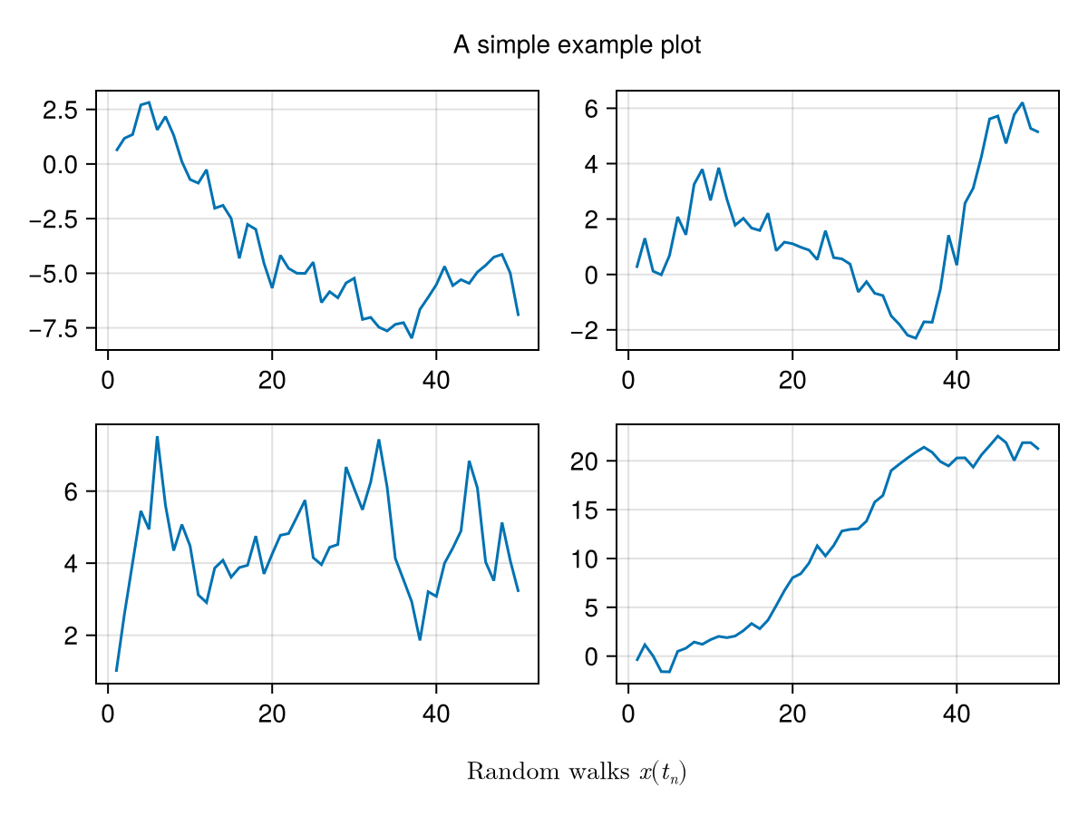

Now we define a theme which changes the default fontsize, activate it, and plot.

fontsize_theme = Theme(fontsize = 10)
set_theme!(fontsize_theme)

example_plot()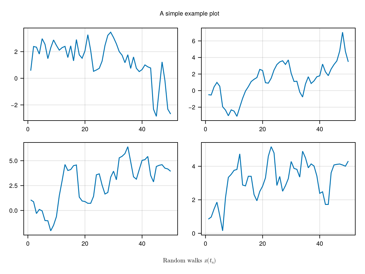

This theme will be active until we call set_theme!().

set_theme!()

merge

Themes often only affect part of the plot attributes. Therefore it is possible to combine themes to get their respective effects together.

For example, you can combine the dark theme with the LaTeX fonts theme to have both the dark colors and uniform fonts.

dark_latexfonts = merge(theme_dark(), theme_latexfonts())
with_theme(dark_latexfonts) do
    example_plot()
end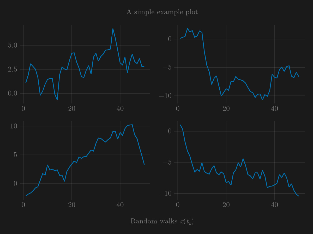

update_theme!

If you have activated a theme already and want to update it partially, without removing the attributes not in the new theme, you can use update_theme!.

For example, you can decide to change the text size after activating the dark and latex theme in the previous section.

update_theme!(fontsize=30)
example_plot()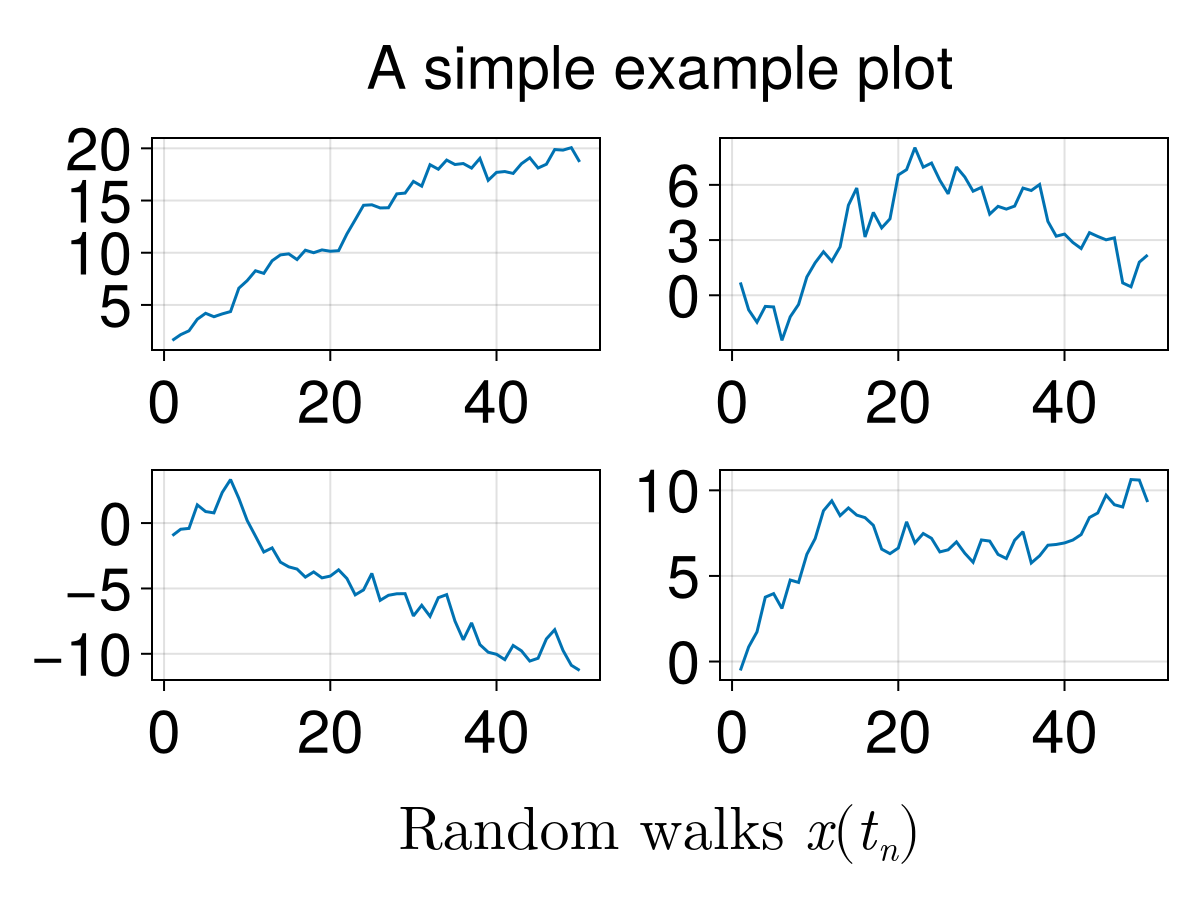

with_theme

Because it can be tedious to remember to switch themes off which you need only temporarily, there's the function with_theme(f, theme) which handles the resetting for you automatically, even if you encounter an error while running f.

with_theme(fontsize_theme) do
    example_plot()
end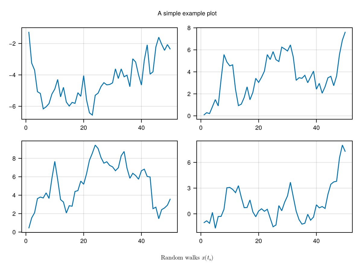

You can also pass additional keywords to add or override attributes in your theme:

with_theme(fontsize_theme, fontsize = 25) do
    example_plot()
end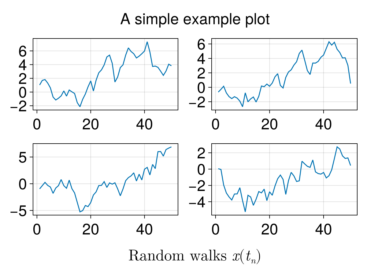

Theming plot objects

You can theme plot objects by using their uppercase type names as a key in your theme.

lines_theme = Theme(
    Lines = (
        linewidth = 4,
        linestyle = :dash,
    )
)

with_theme(example_plot, lines_theme)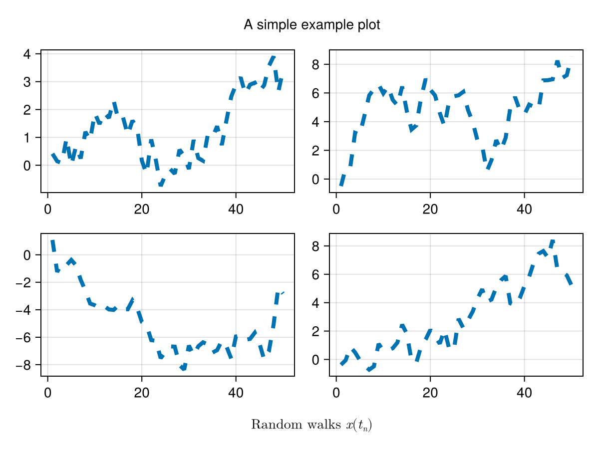

Theming block objects

Every Block such as Axis, Legend, Colorbar, etc. can be themed by using its type name as a key in your theme.

Here is how you could define a simple ggplot-like style for your axes:

ggplot_theme = Theme(
    Axis = (
        backgroundcolor = :gray90,
        leftspinevisible = false,
        rightspinevisible = false,
        bottomspinevisible = false,
        topspinevisible = false,
        xgridcolor = :white,
        ygridcolor = :white,
    )
)

with_theme(example_plot, ggplot_theme)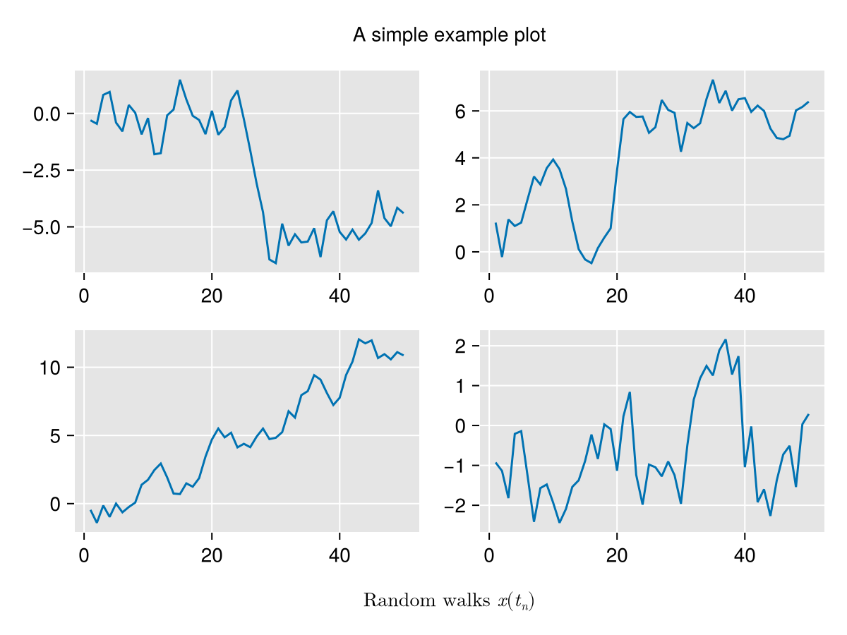

Cycles

Makie supports a variety of options for cycling plot attributes automatically. For a plot object to use cycling, either its default theme or the currently active theme must have the cycle attribute set.

There are multiple ways to specify this attribute:

# You can either make a list of symbols
cycle = [:color, :marker]
# or map specific plot attributes to palette attributes
cycle = [:linecolor => :color, :marker]
# you can also map multiple attributes that should receive
# the same cycle attribute
cycle = [[:linecolor, :markercolor] => :color, :marker]
# nothing disables cycling
cycle = nothing # equivalent to cycle = []

Notice that cycles must be given as attributes to a plot object, not the top-level theme (because different plot objects can cycle different attributes, e.g., a density plot cannot cycle markers). This is exemplified in the following code blocks.

with_theme(
    Theme(
        palette = (color = [:red, :blue], marker = [:circle, :xcross]),
        Scatter = (cycle = [:color, :marker],)
    )) do
    scatter(fill(1, 10))
    scatter!(fill(2, 10))
    scatter!(fill(3, 10))
    scatter!(fill(4, 10))
    scatter!(fill(5, 10))
    current_figure()
end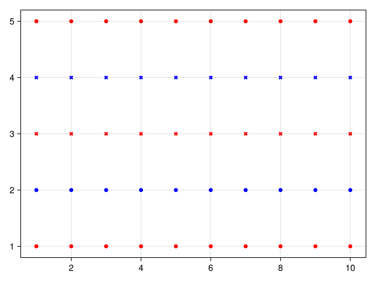

Covarying cycles

You can also construct a Cycle object directly, which additionally allows to set the covary keyword, that defaults to false. A cycler with covary = true cycles all attributes together, instead of cycling through all values of the first, then the second, etc.

# palettes: color = [:red, :blue, :green] marker = [:circle, :rect, :utriangle, :dtriangle]

cycle = [:color, :marker]
# 1: :red, :circle
# 2: :blue, :circle
# 3: :green, :circle
# 4: :red, :rect
# ...

cycle = Cycle([:color, :marker], covary = true)
# 1: :red, :circle
# 2: :blue, :rect
# 3: :green, :utriangle
# 4: :red, :dtriangle
# ...

For example

with_theme(
    Theme(
        palette = (color = [:red, :blue], linestyle = [:dash, :dot]),
        Lines = (cycle = Cycle([:color, :linestyle], covary = true),)
    )) do
    lines(fill(5, 10))
    lines!(fill(4, 10))
    lines!(fill(3, 10))
    lines!(fill(2, 10))
    lines!(fill(1, 10))
    current_figure()
end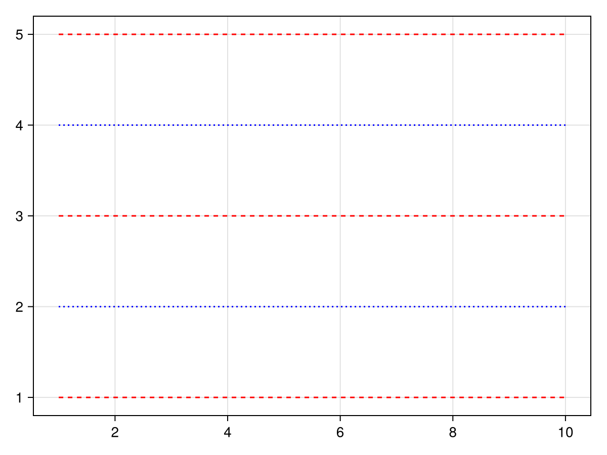

Manual cycling using Cycled

If you want to give a plot's attribute a specific value from the respective cycler, you can use the Cycled object. The index i passed to Cycled is used directly to look up a value in the cycler that belongs to the attribute, and errors if no such cycler is defined. For example, to access the third color in a cycler, instead of plotting three plots to advance the cycler, you can use color = Cycled(3).

The cycler's internal counter is not advanced when using Cycled for any attribute, and only attributes with Cycled access the cycled values, all other usually cycled attributes fall back to their non-cycled defaults.

using CairoMakie
f = Figure()

Axis(f[1, 1])

# the normal cycle
lines!(0..10, x -> sin(x) - 1)
lines!(0..10, x -> sin(x) - 2)
lines!(0..10, x -> sin(x) - 3)

# manually specified colors
lines!(0..10, x -> sin(x) - 5, color = Cycled(3))
lines!(0..10, x -> sin(x) - 6, color = Cycled(2))
lines!(0..10, x -> sin(x) - 7, color = Cycled(1))

f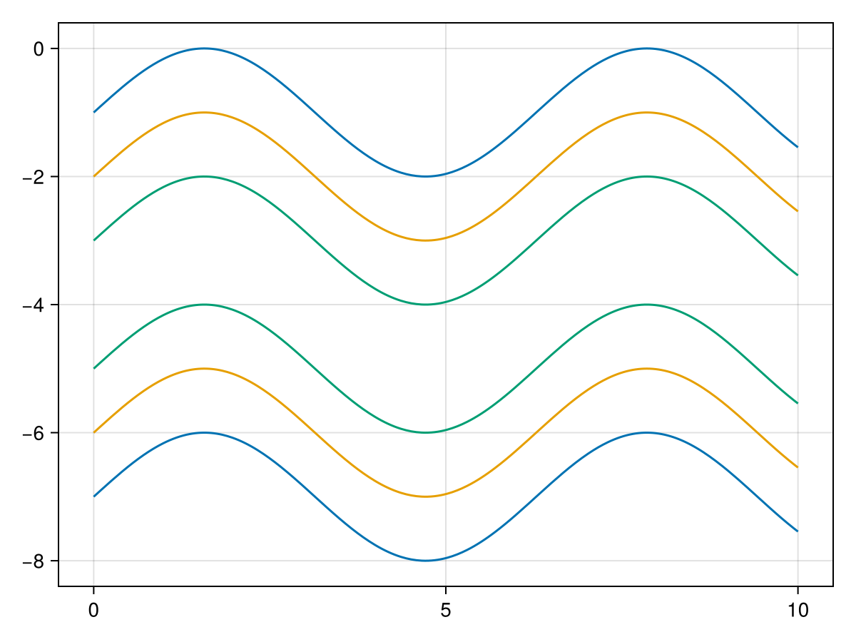

Palettes

The attributes specified in the cycle are looked up in the axis' palette. A single :color is both plot attribute as well as palette attribute, while :color => :patchcolor means that plot.color should be set to palette.patchcolor. Here's an example that shows how density plots react to different palette options:

using CairoMakie

f = Figure(size = (800, 800))

Axis(f[1, 1], title = "Default cycle palette")

for i in 1:6
    density!(randn(50) .+ 2i)
end

Axis(f[2, 1],
    title = "Custom cycle palette",
    palette = (patchcolor = [:red, :green, :blue, :yellow, :orange, :pink],))

for i in 1:6
    density!(randn(50) .+ 2i)
end

set_theme!(Density = (cycle = [],))

Axis(f[3, 1], title = "No cycle")

for i in 1:6
    density!(randn(50) .+ 2i)
end


f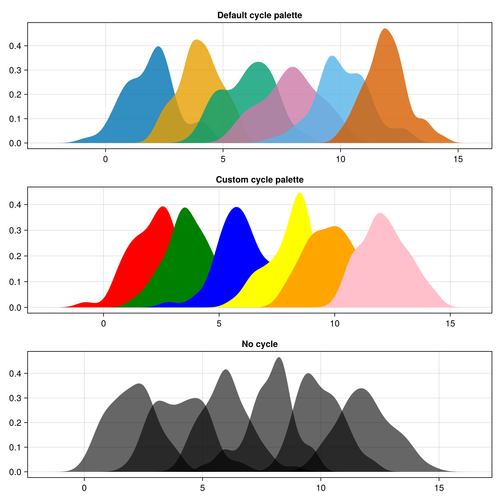

You can also theme global palettes via set_theme!(palette = (color = my_colors, marker = my_markers)) for example.

Special attributes

You can use the keys rowgap and colgap to change the default grid layout gaps.