datashader
Makie.datashader Function
datashader(points::AbstractVector{<: Point})Warning
This feature might change outside breaking releases, since the API is not yet finalized. Please be wary of bugs in the implementation and open issues if you encounter odd behaviour.
Points can be any array type supporting iteration & getindex, including memory mapped arrays. If you have separate arrays for x and y coordinates and want to avoid conversion and copy, consider using:
using Makie.StructArrays
points = StructArray{Point2f}((x, y))
datashader(points)
Do pay attention though, that if x and y don't have a fast iteration/getindex implemented, this might be slower than just copying the data into a new array.
For best performance, use method=Makie.AggThreads() and make sure to start julia with julia -tauto or have the environment variable JULIA_NUM_THREADS set to the number of cores you have.
Plot type
The plot type alias for the datashader function is DataShader.
Examples
Airports
using GLMakie
using DelimitedFiles

airports = Point2f.(eachrow(readdlm(assetpath("airportlocations.csv"))))
fig, ax, ds = datashader(airports,
    colormap=[:white, :black],
    # for documentation output we shouldn't calculate the image async,
    # since it won't wait for the render to finish and inline a blank image
    async = false,
    figure = (; figure_padding=0, size=(360*2, 160*2))
)
Colorbar(fig[1, 2], ds, label="Number of airports")
hidedecorations!(ax); hidespines!(ax)
fig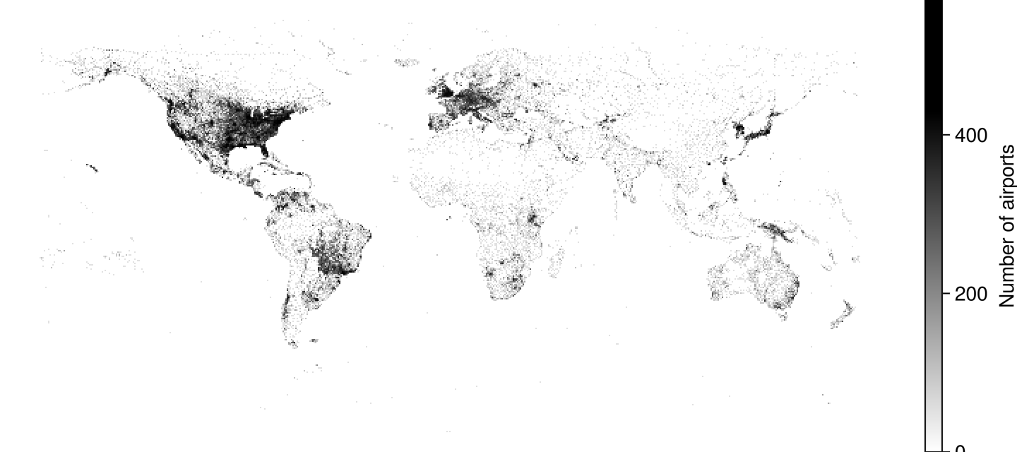
Mean aggregation
The AggMean aggregation type requires Point3s where the mean is taken over the z values of all points that fall into the same x/y bin.
using GLMakie
with_z(p2) = Point3f(p2..., cos(p2[1]) * sin(p2[2]))
points = randn(Point2f, 100_000)
points_with_z = map(with_z, points)

f = Figure()
ax = Axis(f[1, 1], title = "AggMean")
datashader!(ax, points_with_z, agg = Makie.AggMean(), operation = identity)
ax2 = Axis(f[1, 2], title = "AggMean binsize = 3")
datashader!(ax2, points_with_z, agg = Makie.AggMean(), operation = identity, binsize = 3)
f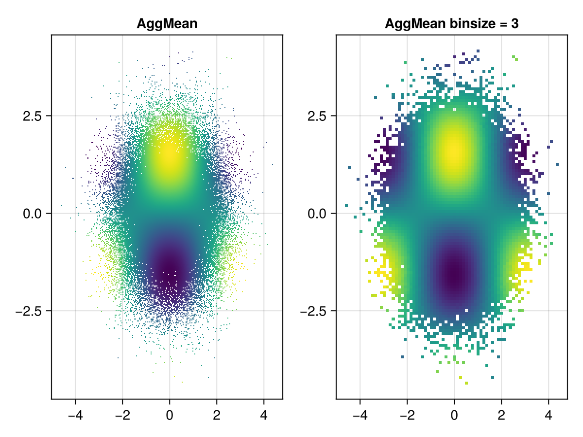
Strange Attractors
using GLMakie
# Taken from Lazaro Alonso in Beautiful Makie:
# https://beautiful.makie.org/dev/examples/generated/2d/datavis/strange_attractors/?h=cliffo#trajectory
Clifford((x, y), a, b, c, d) = Point2f(sin(a * y) + c * cos(a * x), sin(b * x) + d * cos(b * y))

function trajectory(fn, x0, y0, kargs...; n=1000) #  kargs = a, b, c, d
    xy = zeros(Point2f, n + 1)
    xy[1] = Point2f(x0, y0)
    @inbounds for i in 1:n
        xy[i+1] = fn(xy[i], kargs...)
    end
    return xy
end

cargs = [[0, 0, -1.3, -1.3, -1.8, -1.9],
    [0, 0, -1.4, 1.6, 1.0, 0.7],
    [0, 0, 1.7, 1.7, 0.6, 1.2],
    [0, 0, 1.7, 0.7, 1.4, 2.0],
    [0, 0, -1.7, 1.8, -1.9, -0.4],
    [0, 0, 1.1, -1.32, -1.03, 1.54],
    [0, 0, 0.77, 1.99, -1.31, -1.45],
    [0, 0, -1.9, -1.9, -1.9, -1.0],
    [0, 0, 0.75, 1.34, -1.93, 1.0],
    [0, 0, -1.32, -1.65, 0.74, 1.81],
    [0, 0, -1.6, 1.6, 0.7, -1.0],
    [0, 0, -1.7, 1.5, -0.5, 0.7]
]

fig = Figure(size=(1000, 1000))
fig_grid = CartesianIndices((3, 4))
cmap = to_colormap(:BuPu_9)
cmap[1] = RGBAf(1, 1, 1, 1) # make sure background is white

let
    # locally, one can go pretty high with n_points,
    # e.g. 4*(10^7), but we don't want the docbuild to become too slow.
    n_points = 10^6
    for (i, arg) in enumerate(cargs)
        points = trajectory(Clifford, arg...; n=n_points)
        r, c = Tuple(fig_grid[i])
        ax, plot = datashader(fig[r, c], points;
            colormap=cmap,
            async=false,
            axis=(; title=join(string.(arg), ", ")))
        hidedecorations!(ax)
        hidespines!(ax)
    end
end
rowgap!(fig.layout,5)
colgap!(fig.layout,1)
fig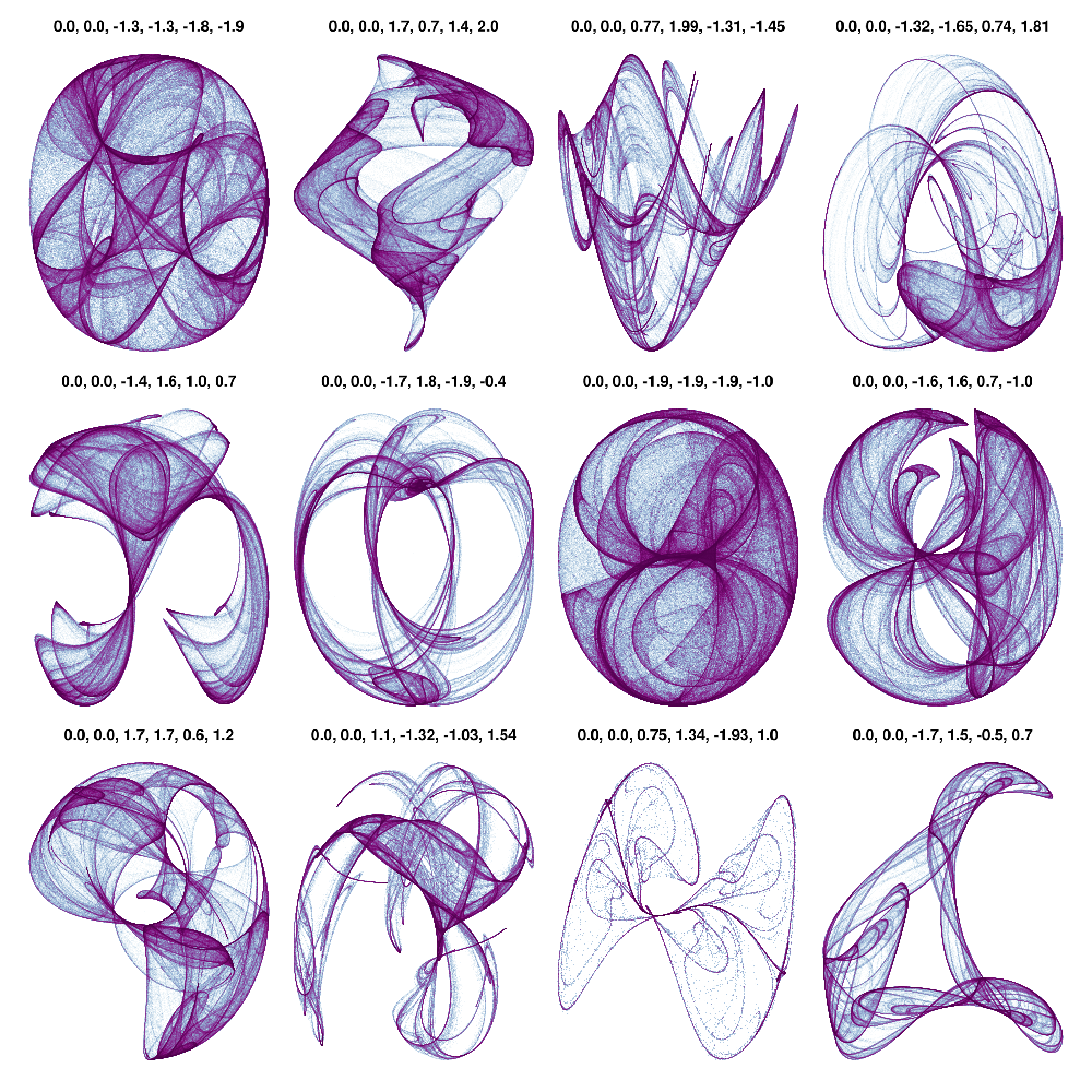
Bigger examples
Timings in the comments are from running this on a 32gb Ryzen 5800H laptop. Both examples aren't fully optimized yet, and just use raw, unsorted, memory mapped Point2f arrays. In the future, we'll want to add acceleration structures to optimize access to sub-regions.
14 million point NYC taxi dataset
using GLMakie, Downloads, Parquet2
bucket = "https://ursa-labs-taxi-data.s3.us-east-2.amazonaws.com"
year = 2009
month = "01"
filename = join([year, month, "data.parquet"], "/")
out = joinpath("$year-$month-data.parquet")
url = bucket * "/" * filename
Downloads.download(url, out)
# Loading ~1.5s
@time begin
    ds = Parquet2.Dataset(out)
    dlat = Parquet2.load(ds, "dropoff_latitude")
    dlon = Parquet2.load(ds, "dropoff_longitude")
    # One could use struct array here, but dlon/dlat are
    # a custom array type from Parquet2 supporting missing and some other things, which slows the whole thing down.
    # points = StructArray{Point2f}((dlon, dlat))
    points = Point2f.(dlon, dlat)
    groups = Parquet2.load(ds, "vendor_id")
end

# ~0.06s
@time begin
    f, ax, dsplot = datashader(points;
        colormap=:fire,
        axis=(; type=Axis, autolimitaspect = 1),
        figure=(;figure_padding=0, size=(1200, 600))
    )
    # Zoom into the hotspot
    limits!(ax, Rect2f(-74.175, 40.619, 0.5, 0.25))
    # make image fill the whole screen
    hidedecorations!(ax)
    hidespines!(ax)
    display(f)
end
2.7 billion OSM GPS points
Download the data from OSM GPS points and use the updated script from drawing-2-7-billion-points-in-10s to convert the CSV to a binary blob that we can memory map.
using GLMakie, Mmap
path = "gpspoints.bin"

points = Mmap.mmap(open(path, "r"), Vector{Point2f});
# ~ 26s
@time begin
    f, ax, pl = datashader(
        points;
        # For a big dataset its interesting to see how long each aggregation takes
        show_timings = true,
        # Use a local operation which is faster to calculate and looks good!
        local_operation=x-> log10(x + 1),
        #=
            in the code we used to save the binary, we had the points in the wrong order.
            A good chance to demonstrate the `point_transform` argument,
            Which gets applied to every point before aggregating it
        =#
        point_transform=reverse,
        axis=(; type=Axis, autolimitaspect = 1),
        figure=(;figure_padding=0, size=(1200, 600))
    )
    hidedecorations!(ax)
    hidespines!(ax)
    display(f)
end
aggregation took 1.395s
aggregation took 1.176s
aggregation took 0.81s
aggregation took 0.791s
aggregation took 0.729s
aggregation took 1.272s
aggregation took 1.117s
aggregation took 0.866s
aggregation took 0.724sCategorical Data
There are two ways to plot categorical data right now:
datashader(one_category_per_point, points)
datashader(Dict(:category_a => all_points_a, :category_b => all_points_b))
The type of the category doesn't matter, but will get converted to strings internally, to be displayed nicely in the legend. Categories are currently aggregated in one Canvas per category, and then overlaid with alpha blending.
using GLMakie
normaldist = randn(Point2f, 1_000_000)
ds1 = normaldist .+ (Point2f(-1, 0),)
ds2 = normaldist .+ (Point2f(1, 0),)
fig, ax, pl = datashader(Dict("a" => ds1, "b" => ds2); async = false)
hidedecorations!(ax)
fig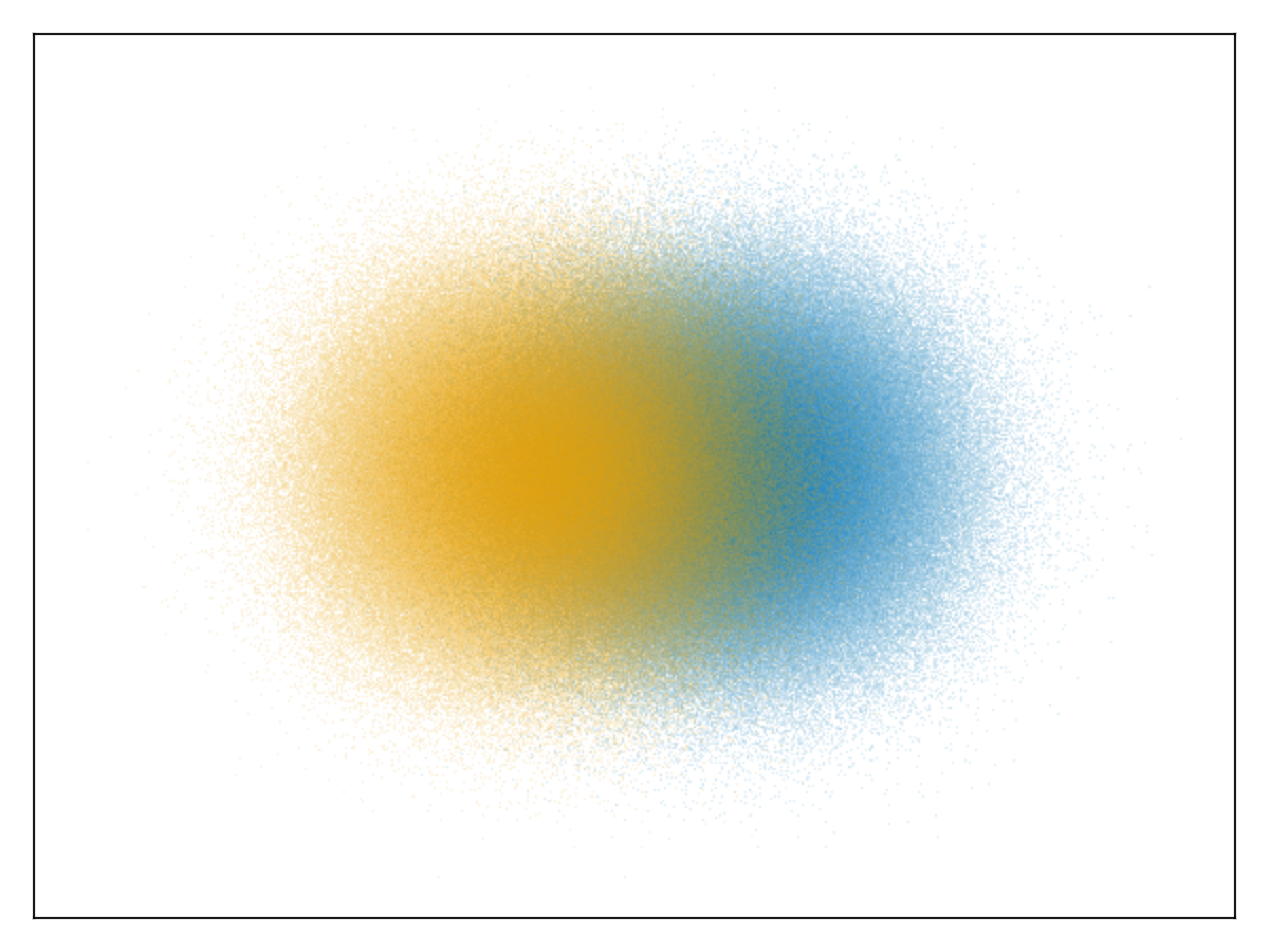
We can also re-use the previous NYC example for a categorical plot:
@time begin
    f = Figure(figure_padding=0, size=(1200, 600))
    ax = Axis(
        f[1, 1],
        autolimitaspect=1,
        limits=(-74.022, -73.827, 40.696, 40.793),
        backgroundcolor=:black
    )
    datashader!(ax, groups, points)
    hidedecorations!(ax)
    hidespines!(ax)
    # Create a styled legend
    axislegend("Vendor ID"; titlecolor=:white, framecolor=:grey, polystrokewidth=2, polystrokecolor=(:white, 0.5), rowgap=10, backgroundcolor=:black, labelcolor=:white)
    display(f)
end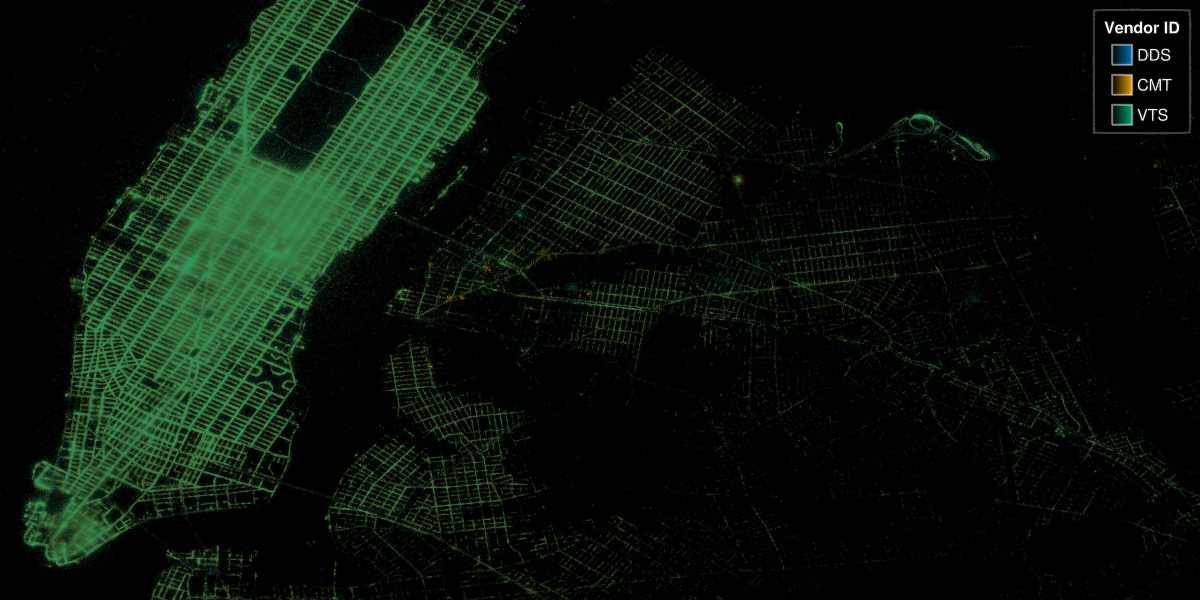
Advanced API
The datashader recipe makes it very simple to get started, and is also efficiently implemented so that most changes like f, ax, pl = datashader(...); pl.colorrange=new_range; pl.operation=log10 won't redo the aggregation. But if you still need more manual control, one can also use the underlying Canvas API directly for more manual control:
Attributes
agg
Defaults to AggCount{Float32}()
Can be AggCount(), AggAny() or AggMean(). Be sure, to use the correct element type e.g. AggCount{Float32}(), which needs to accommodate the output of local_operation. User-extensible by overloading:
struct MyAgg{T} <: Makie.AggOp end
MyAgg() = MyAgg{Float64}()
Makie.Aggregation.null(::MyAgg{T}) where {T} = zero(T)
Makie.Aggregation.embed(::MyAgg{T}, x) where {T} = convert(T, x)
Makie.Aggregation.merge(::MyAgg{T}, x::T, y::T) where {T} = x + y
Makie.Aggregation.value(::MyAgg{T}, x::T) where {T} = x
alpha
Defaults to 1.0
The alpha value of the colormap or color attribute. Multiple alphas like in plot(alpha=0.2, color=(:red, 0.5), will get multiplied.
async
Defaults to true
Will calculate get_aggregation in a task, and skip any zoom/pan updates while busy. Great for interaction, but must be disabled for saving to e.g. png or when inlining in Documenter.
binsize
Defaults to 1
Factor defining how many bins one wants per screen pixel. Set to n > 1 if you want a coarser image.
clip_planes
Defaults to automatic
Clip planes offer a way to do clipping in 3D space. You can set a Vector of up to 8 Plane3f planes here, behind which plots will be clipped (i.e. become invisible). By default clip planes are inherited from the parent plot or scene. You can remove parent clip_planes by passing Plane3f[].
colormap
Defaults to @inherit colormap :viridis
Sets the colormap that is sampled for numeric colors. PlotUtils.cgrad(...), Makie.Reverse(any_colormap) can be used as well, or any symbol from ColorBrewer or PlotUtils. To see all available color gradients, you can call Makie.available_gradients().
colorrange
Defaults to automatic
The values representing the start and end points of colormap.
colorscale
Defaults to identity
The color transform function. Can be any function, but only works well together with Colorbar for identity, log, log2, log10, sqrt, logit, Makie.pseudolog10 and Makie.Symlog10.
depth_shift
Defaults to 0.0
adjusts the depth value of a plot after all other transformations, i.e. in clip space, where 0 <= depth <= 1. This only applies to GLMakie and WGLMakie and can be used to adjust render order (like a tunable overdraw).
fxaa
Defaults to true
adjusts whether the plot is rendered with fxaa (anti-aliasing, GLMakie only).
highclip
Defaults to automatic
The color for any value above the colorrange.
inspectable
Defaults to true
sets whether this plot should be seen by DataInspector.
inspector_clear
Defaults to automatic
Sets a callback function (inspector, plot) -> ... for cleaning up custom indicators in DataInspector.
inspector_hover
Defaults to automatic
Sets a callback function (inspector, plot, index) -> ... which replaces the default show_data methods.
inspector_label
Defaults to automatic
Sets a callback function (plot, index, position) -> string which replaces the default label generated by DataInspector.
interpolate
Defaults to false
If the resulting image should be displayed interpolated. Note that interpolation can make NaN-adjacent bins also NaN in some backends, for example due to interpolation schemes used in GPU hardware. This can make it look like there are more NaN bins than there actually are.
local_operation
Defaults to identity
Function which gets called on each element after the aggregation (map!(x-> local_operation(x), final_aggregation_result)).
lowclip
Defaults to automatic
The color for any value below the colorrange.
method
Defaults to AggThreads()
Can be AggThreads() or AggSerial() for threaded vs. serial aggregation.
model
Defaults to automatic
Sets a model matrix for the plot. This overrides adjustments made with translate!, rotate! and scale!.
nan_color
Defaults to :transparent
The color for NaN values.
operation
Defaults to automatic
Defaults to Makie.equalize_histogram function which gets called on the whole get_aggregation array before display (operation(final_aggregation_result)).
overdraw
Defaults to false
Controls if the plot will draw over other plots. This specifically means ignoring depth checks in GL backends
point_transform
Defaults to identity
Function which gets applied to every point before aggregating it.
show_timings
Defaults to false
Set to true to show how long it takes to aggregate each frame.
space
Defaults to :data
sets the transformation space for box encompassing the plot. See Makie.spaces() for possible inputs.
ssao
Defaults to false
Adjusts whether the plot is rendered with ssao (screen space ambient occlusion). Note that this only makes sense in 3D plots and is only applicable with fxaa = true.
transformation
Defaults to automatic
No docs available.
transparency
Defaults to false
Adjusts how the plot deals with transparency. In GLMakie transparency = true results in using Order Independent Transparency.
visible
Defaults to true
Controls whether the plot will be rendered or not.