
mesh
MakieCore.mesh Function
mesh(x, y, z)
mesh(mesh_object)
mesh(x, y, z, faces)
mesh(xyz, faces)
Plots a 3D or 2D mesh. Supported mesh_objects include Mesh types from GeometryBasics.jl.
Plot type
The plot type alias for the mesh function is Mesh.
Examples
Simple mesh plots
A mesh can be constructed from a set of vertex coordinates and faces.
using GLMakie
vertices = [
    0.0 0.0;
    1.0 0.0;
    1.0 1.0;
    0.0 1.0;
]

faces = [
    1 2 3;
    3 4 1;
]

colors = [:red, :green, :blue, :orange]

mesh(vertices, faces, color = colors, shading = NoShading)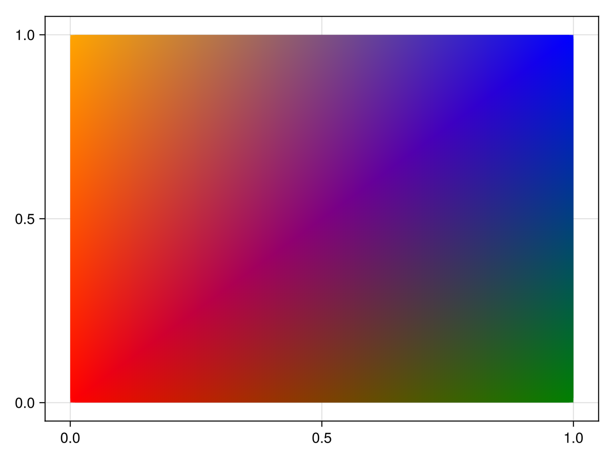
Note that the order of vertices within a face matters for normal generation in 3D and thus affects shading. The normals follows the right hand rule, meaning the normals will face outwards if the vertices of a face are in a counter clockwise order.
using GLMakie
vertices = Point3f[(1,0,0), (1,1,0), (0,1,0)]
faces1 = [1 2 3]
faces2 = [1 3 2]
colors = [:red, :green, :blue]

f = Figure(size = (800, 400))
ax = LScene(f[1,1], show_axis = false)
p = mesh!(ax, vertices, faces1, color = colors)
arrows!(ax, vertices, p.converted[1][].normal, lengthscale = 0.1, arrowsize = Vec3f(0.05, 0.05, 0.1), color = :orange)
text!(ax, vertices[faces1[:]], text = ["1", "2", "3"], align = (:center, :center), fontsize = 20, strokecolor = :white, strokewidth = 2, overdraw = true)

ax = LScene(f[1,2], show_axis = false)
p = mesh!(ax, vertices, faces2, color = colors)
arrows!(ax, vertices, p.converted[1][].normal, lengthscale = 0.1, arrowsize = Vec3f(0.05, 0.05, 0.1), color = :orange)
text!(ax, vertices[faces2[:]], text = ["1", "2", "3"], align = (:center, :center), fontsize = 20, strokecolor = :white, strokewidth = 2, overdraw = true)

f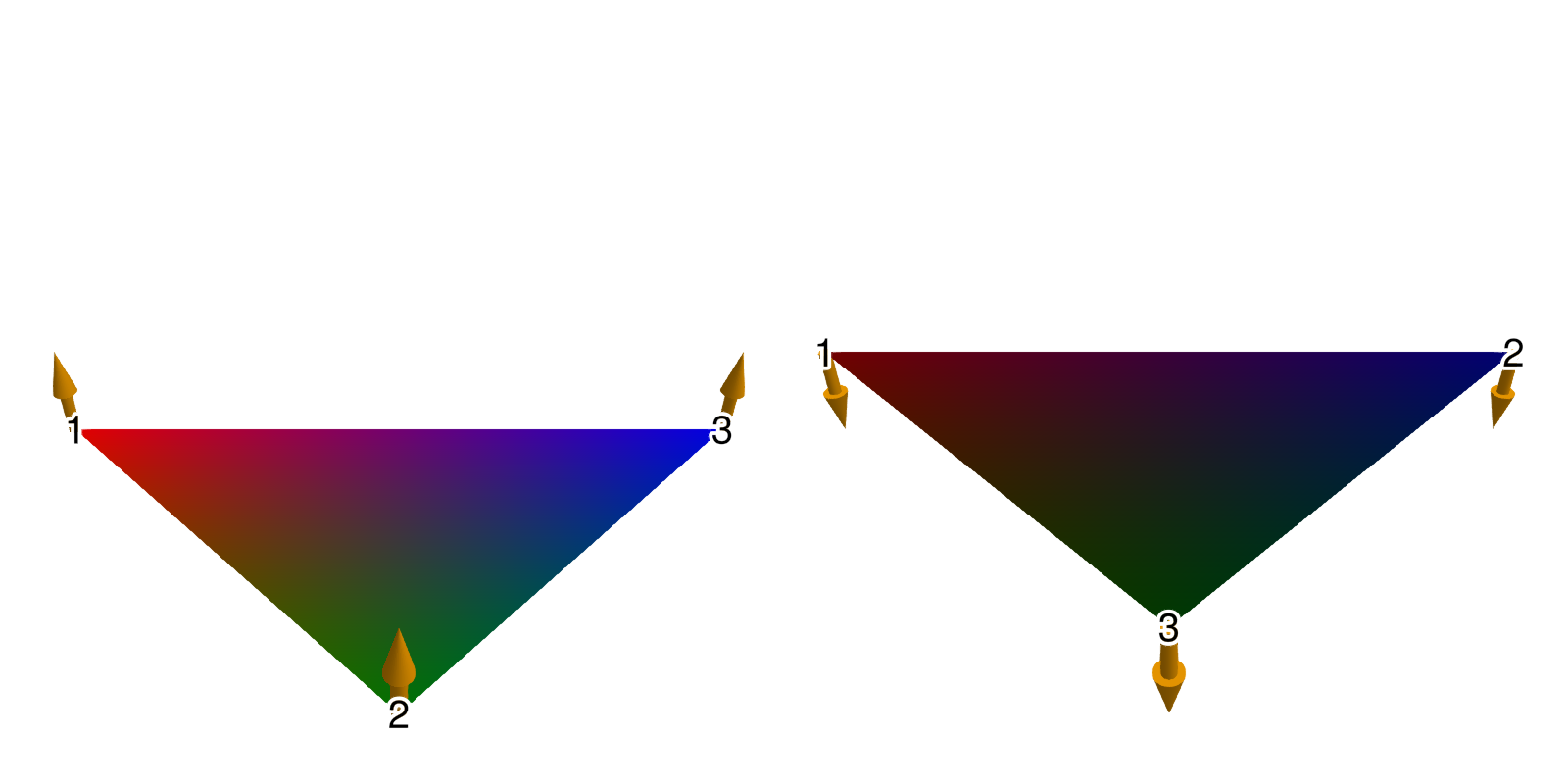
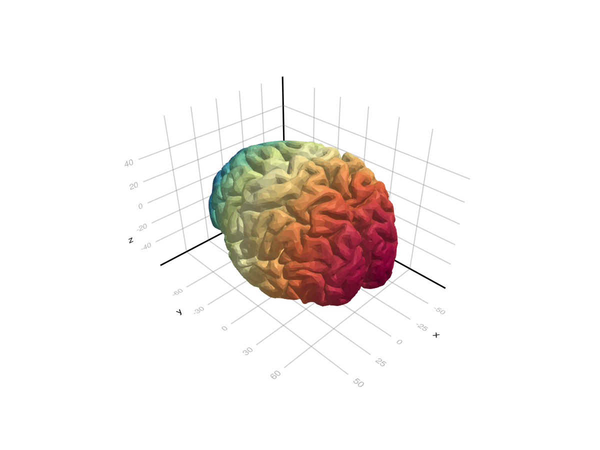
Another quick way to create a mesh plot is import a mesh using FileIO (which relies on MeshIO):
using GLMakie
using FileIO

brain = load(assetpath("brain.stl"))

mesh(
    brain,
    color = [tri[1][2] for tri in brain for i in 1:3],
    colormap = Reverse(:Spectral)
)
Face colors and normals
using GLMakie
using GeometryBasics

# Reduce quality of sphere
s = Tessellation(Sphere(Point3f(0), 1f0), 12)
ps = coordinates(s)
fs = faces(s)

# Use a FaceView to with a new set of faces which refer to one color per face.
# Each face must have the same length as the respective face in fs.
# (Using the same face type guarantees this)
FT = eltype(fs); N = length(fs)
cs = FaceView(rand(RGBf, N), [FT(i) for i in 1:N])

# generate normals per face (this creates a FaceView as well)
ns = face_normals(ps, fs)

# Create mesh
m = GeometryBasics.mesh(ps, fs, normal = ns, color = cs)

mesh(m)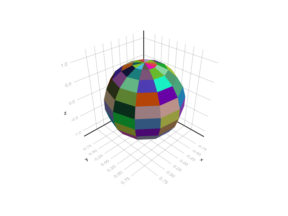
Using GeometryBasics.Mesh and Buffer/Sampler type
We can also create a mesh to specify normals, uv coordinates:
using GeometryBasics, LinearAlgebra, GLMakie, FileIO


# Create vertices for a Sphere
r = 0.5f0
n = 30
θ = LinRange(0, pi, n)
φ2 = LinRange(0, 2pi, 2 * n)
x2 = [r * cos(φv) * sin(θv) for θv in θ, φv in φ2]
y2 = [r * sin(φv) * sin(θv) for θv in θ, φv in φ2]
z2 = [r * cos(θv) for θv in θ, φv in 2φ2]
points = vec([Point3f(xv, yv, zv) for (xv, yv, zv) in zip(x2, y2, z2)])

# The coordinates form a matrix, so to connect neighboring vertices with a face
# we can just use the faces of a rectangle with the same dimension as the matrix:
_faces = decompose(QuadFace{GLIndex}, Tessellation(Rect(0, 0, 1, 1), size(z2)))
# Normals of a centered sphere are easy, they're just the vertices normalized.
_normals = normalize.(points)

# Now we generate UV coordinates, which map the image (texture) to the vertices.
# (0, 0) means lower left edge of the image, while (1, 1) means upper right corner.
function gen_uv(shift)
    return vec(map(CartesianIndices(size(z2))) do ci
        tup = ((ci[1], ci[2]) .- 1) ./ ((size(z2) .* shift) .- 1)
        return Vec2f(reverse(tup))
    end)
end

# We add some shift to demonstrate how UVs work:
uv = gen_uv(0.0)
# We can use a Buffer to update single elements in an array directly on the GPU
# with GLMakie. They work just like normal arrays, but forward any updates written to them directly to the GPU
uv_buff = Buffer(uv)
gb_mesh = GeometryBasics.Mesh(points, _faces; uv = uv_buff, normal = _normals)

f, ax, pl = mesh(gb_mesh,  color = rand(100, 100), colormap=:blues)
wireframe!(ax, gb_mesh, color=(:black, 0.2), linewidth=2, transparency=true)
record(f, "uv_mesh.mp4", LinRange(0, 1, 100)) do shift
    uv_buff[1:end] = gen_uv(shift)
end
The uv coordinates that go out of bounds will get repeated per default. One can use a Sampler object to change that behaviour:
#=
Possible values:
:clamp_to_edge (default)
:mirrored_repeat
:repeat
=#
data = load(Makie.assetpath("earth.png"))
color = Sampler(rotl90(data'), x_repeat=:mirrored_repeat,y_repeat=:repeat)
f, ax, pl = mesh(gb_mesh,  color = color)
wireframe!(ax, gb_mesh, color=(:black, 0.2), linewidth=2, transparency=true)

record(f, "uv_mesh_mirror.mp4", LinRange(0, 1, 100)) do shift
    uv_buff[1:end] = gen_uv(shift)
end
Volume Texture
One can pass a 3d array to `mesh(args...; color=volume), and index the volume via uvw coordinates. Here is an example of an interactive volume slice viewer:
using GLMakie, GeometryBasics, NIfTI
brain = Float32.(niread(Makie.assetpath("brain.nii.gz")).raw)
# Define the positions
positions = Observable([Point3f(0.5, 0, 0), Point3f(0.5, 1, 0), Point3f(0.5, 1, 1), Point3f(0.5, 0, 1)])
triangles = GLTriangleFace[(1, 2, 3), (3, 4, 1)]

# We will stay in the unit cube, so the uv coordinates are just the positions.
uv_mesh = map((p) -> GeometryBasics.Mesh(p, triangles; uv=Vec3f.(p)), positions)
# Pass the volume plot to the color
f, ax, pl = mesh(uv_mesh, color=brain, shading=NoShading, axis=(; show_axis=false))
# Visualize the unit cube in which the volume lives
wireframe!(ax, Rect3f(Vec3f(0), Vec3f(1)), transparency=true, color=(:gray, 0.5))
cam = cameracontrols(ax.scene)
# Only rotate when left + alt buttons are pressed, so we can better interact with the slice
cam.controls.rotation_button = Mouse.left & Keyboard.left_alt
# Have colors for each point, so we can highlight it on hover
colors = Observable(fill(:black, 4))
ms = meshscatter!(ax, positions, markersize=0.05, color=colors)
# Also plot the volume next to it with a maximum intensity projection.
Makie.volume(f[1, 2], brain)

# Use mouseevents for drag events etc.
m_events = addmouseevents!(ax.scene)
point_idx = Ref(0)
point_start = Ref(Point3f(0))
clear_color() = if any(x -> x == :red, colors[])
    colors[] .= :black
    notify(colors)
end
# Define the handler for handling drag events to move the slice and
# highlight hovered points.
onany(ax.scene.events.mouseposition, m_events.obs) do mp, event
    if event.type == Makie.MouseEventTypes.leftdragstart
        p, idx = Makie.pick(ax.scene)
        if p == ms
            point_idx[] = idx
            colors[][idx] = :red
            point_start[] = positions[][idx]
            notify(colors)
        else
            point_idx[] = 0
        end
    elseif event.type == Makie.MouseEventTypes.leftdrag
        if point_idx[] != 0
            ray = Makie.ray_at_cursor(ax.scene)
            p = point_start[]
            line_start = Point3f(0, p[2], p[3])
            line_end = Point3f(1, p[2], p[3])
            new_point = Makie.closest_point_on_line(line_start, line_end, ray)
            positions[][point_idx[]] = new_point
            notify(positions)
        end
    elseif event.type == Makie.MouseEventTypes.leftdragstop
        point_idx[] = 0
        clear_color()
    elseif event.type == Makie.MouseEventTypes.over
        p, idx = Makie.pick(ax.scene)
        if p == ms
            if colors[][idx] != :red
                colors[][idx] = :red
                notify(colors)
            end
        else
            clear_color()
            point_idx[] = 0
        end
    end
end
f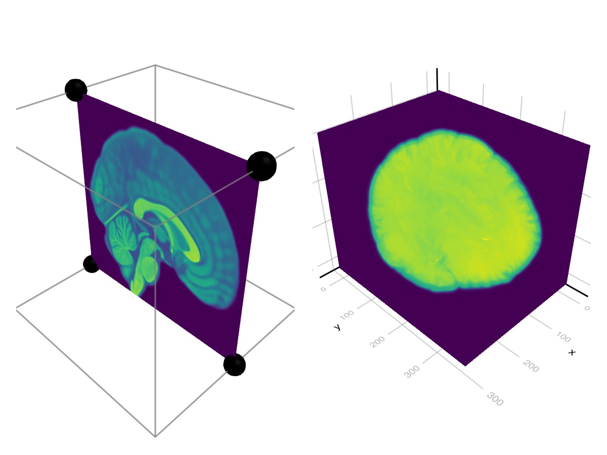
Complex Meshes (Experimental)
using GLMakie
using FileIO

# Load a mesh with material information. This will produce a GeometryBasics.MetaMesh
sponza = load(assetpath("sponza/sponza.obj"))

# The MetaMesh contains a standard GeometryBasics.Mesh in `sponza.mesh` with
# `mesh.views` defining the different sub-meshes, and material metadata in the
# `sponza.meta` Dict. The metadata includes:
# - meta[:material_names] which maps each view in `mesh.views` to a material name
# - meta[:materials] which maps a material name to a nested Dict of the loaded properties
# When a MetaMesh is given to Makie.mesh(), it will look for these entries and
# try to build a plot accordingly.
f, a, p = mesh(sponza)

# Set up camera
update_cam!(a.scene, Vec3f(-15, 7, 1), Vec3f(3, 5, 0), Vec3f(0,1,0))
cameracontrols(a).settings.center[] = false # don't recenter on display
cameracontrols(a).settings.fixed_axis[] = false # rotate freely
f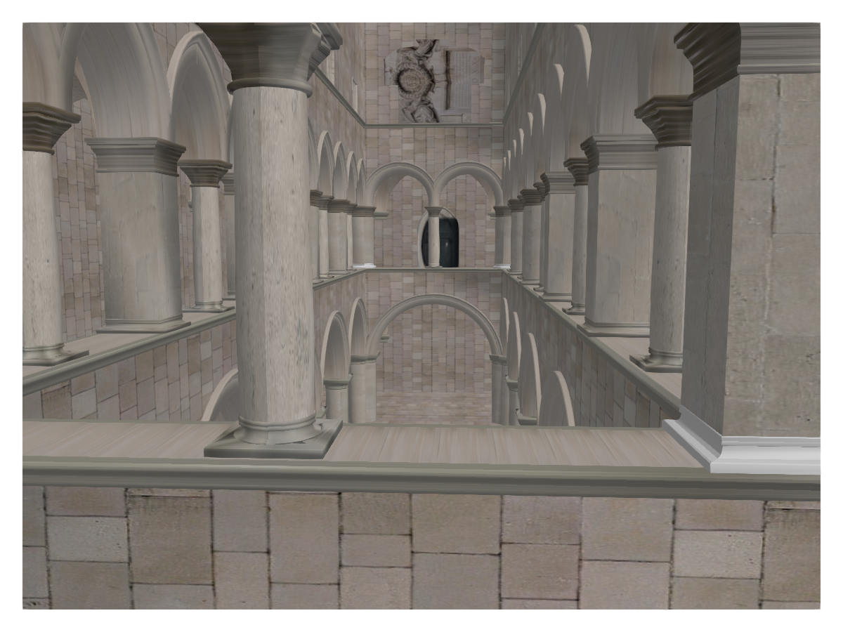
Attributes
alpha
Defaults to 1.0
The alpha value of the colormap or color attribute. Multiple alphas like in plot(alpha=0.2, color=(:red, 0.5), will get multiplied.
backlight
Defaults to 0.0
Sets a weight for secondary light calculation with inverted normals.
clip_planes
Defaults to automatic
Clip planes offer a way to do clipping in 3D space. You can set a Vector of up to 8 Plane3f planes here, behind which plots will be clipped (i.e. become invisible). By default clip planes are inherited from the parent plot or scene. You can remove parent clip_planes by passing Plane3f[].
color
Defaults to @inherit patchcolor
Sets the color of the mesh. Can be a Vector{<:Colorant} for per vertex colors or a single Colorant. A Matrix{<:Colorant} can be used to color the mesh with a texture, which requires the mesh to contain texture coordinates. A <: AbstractPattern can be used to apply a repeated, pixel sampled pattern to the mesh, e.g. for hatching.
colormap
Defaults to @inherit colormap :viridis
Sets the colormap that is sampled for numeric colors. PlotUtils.cgrad(...), Makie.Reverse(any_colormap) can be used as well, or any symbol from ColorBrewer or PlotUtils. To see all available color gradients, you can call Makie.available_gradients().
colorrange
Defaults to automatic
The values representing the start and end points of colormap.
colorscale
Defaults to identity
The color transform function. Can be any function, but only works well together with Colorbar for identity, log, log2, log10, sqrt, logit, Makie.pseudolog10 and Makie.Symlog10.
cycle
Defaults to [:color => :patchcolor]
No docs available.
depth_shift
Defaults to 0.0
Adjusts the depth value of a plot after all other transformations, i.e. in clip space, where -1 <= depth <= 1. This only applies to GLMakie and WGLMakie and can be used to adjust render order (like a tunable overdraw).
diffuse
Defaults to 1.0
Sets how strongly the red, green and blue channel react to diffuse (scattered) light.
fxaa
Defaults to true
Adjusts whether the plot is rendered with fxaa (anti-aliasing, GLMakie only).
highclip
Defaults to automatic
The color for any value above the colorrange.
inspectable
Defaults to @inherit inspectable
Sets whether this plot should be seen by DataInspector. The default depends on the theme of the parent scene.
inspector_clear
Defaults to automatic
Sets a callback function (inspector, plot) -> ... for cleaning up custom indicators in DataInspector.
inspector_hover
Defaults to automatic
Sets a callback function (inspector, plot, index) -> ... which replaces the default show_data methods.
inspector_label
Defaults to automatic
Sets a callback function (plot, index, position) -> string which replaces the default label generated by DataInspector.
interpolate
Defaults to true
sets whether colors should be interpolated
lowclip
Defaults to automatic
The color for any value below the colorrange.
matcap
Defaults to nothing
No docs available.
material
Defaults to nothing
RPRMakie only attribute to set complex RadeonProRender materials. Warning, how to set an RPR material may change and other backends will ignore this attribute
model
Defaults to automatic
Sets a model matrix for the plot. This overrides adjustments made with translate!, rotate! and scale!.
nan_color
Defaults to :transparent
The color for NaN values.
overdraw
Defaults to false
Controls if the plot will draw over other plots. This specifically means ignoring depth checks in GL backends
shading
Defaults to automatic
Sets the lighting algorithm used. Options are NoShading (no lighting), FastShading (AmbientLight + PointLight) or MultiLightShading (Multiple lights, GLMakie only). Note that this does not affect RPRMakie.
shininess
Defaults to 32.0
Sets how sharp the reflection is.
space
Defaults to :data
Sets the transformation space for box encompassing the plot. See Makie.spaces() for possible inputs.
specular
Defaults to 0.2
Sets how strongly the object reflects light in the red, green and blue channels.
ssao
Defaults to false
Adjusts whether the plot is rendered with ssao (screen space ambient occlusion). Note that this only makes sense in 3D plots and is only applicable with fxaa = true.
transformation
Defaults to :automatic
No docs available.
transparency
Defaults to false
Adjusts how the plot deals with transparency. In GLMakie transparency = true results in using Order Independent Transparency.
uv_transform
Defaults to automatic
Sets a transform for uv coordinates, which controls how a texture is mapped to a mesh. The attribute can be I, scale::VecTypes{2}, (translation::VecTypes{2}, scale::VecTypes{2}), any of :rotr90, :rotl90, :rot180, :swap_xy/:transpose, :flip_x, :flip_y, :flip_xy, or most generally a Makie.Mat{2, 3, Float32} or Makie.Mat3f as returned by Makie.uv_transform(). They can also be changed by passing a tuple (op3, op2, op1).
visible
Defaults to true
Controls whether the plot will be rendered or not.