contourf

Makie.contourf Function

contourf(xs, ys, zs; kwargs...)

Plots a filled contour of the height information in zs at horizontal grid positions xs and vertical grid positions ys.

xs and ys can be vectors for rectilinear grids or matrices for curvilinear grids, similar to how surface works.

Plot type

The plot type alias for the contourf function is Contourf.

source

using CairoMakie
using DelimitedFiles


volcano = readdlm(Makie.assetpath("volcano.csv"), ',', Float64)

f = Figure()
Axis(f[1, 1])

co = contourf!(volcano, levels = 10)

Colorbar(f[1, 2], co)

f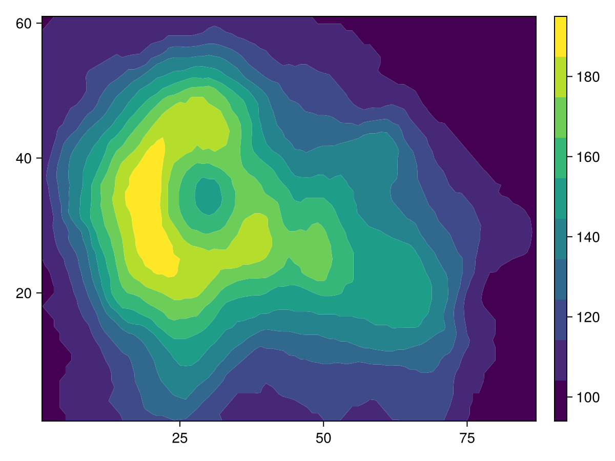

using CairoMakie
using DelimitedFiles


volcano = readdlm(Makie.assetpath("volcano.csv"), ',', Float64)

f = Figure()
ax = Axis(f[1, 1])

co = contourf!(volcano,
    levels = range(100, 180, length = 10),
    extendlow = :cyan, extendhigh = :magenta)

tightlimits!(ax)

Colorbar(f[1, 2], co)

f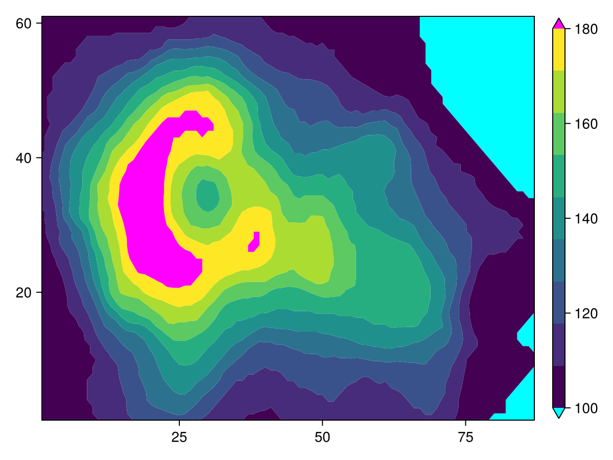

using CairoMakie
using DelimitedFiles


volcano = readdlm(Makie.assetpath("volcano.csv"), ',', Float64)

f = Figure()
ax = Axis(f[1, 1])

co = contourf!(volcano,
    levels = range(100, 180, length = 10),
    extendlow = :auto, extendhigh = :auto)

tightlimits!(ax)

Colorbar(f[1, 2], co)

f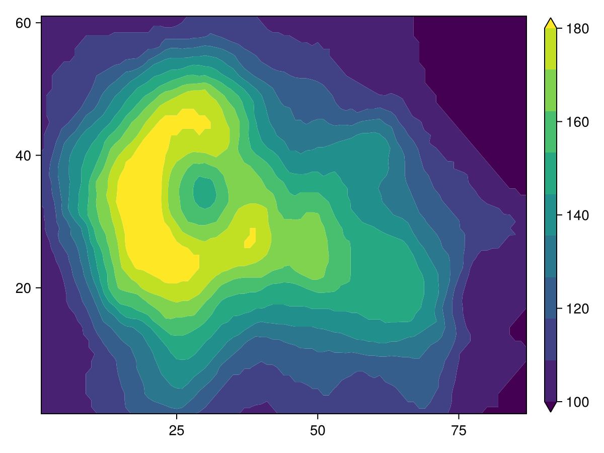

Relative mode

Sometimes it's beneficial to drop one part of the range of values, usually towards the outer boundary. Rather than specifying the levels to include manually, you can set the mode attribute to :relative and specify the levels from 0 to 1, relative to the current minimum and maximum value.

using CairoMakie
using DelimitedFiles


volcano = readdlm(Makie.assetpath("volcano.csv"), ',', Float64)

f = Figure(size = (800, 400))

Axis(f[1, 1], title = "Relative mode, drop lowest 30%")
contourf!(volcano, levels = 0.3:0.1:1, mode = :relative)

Axis(f[1, 2], title = "Normal mode")
contourf!(volcano, levels = 10)

f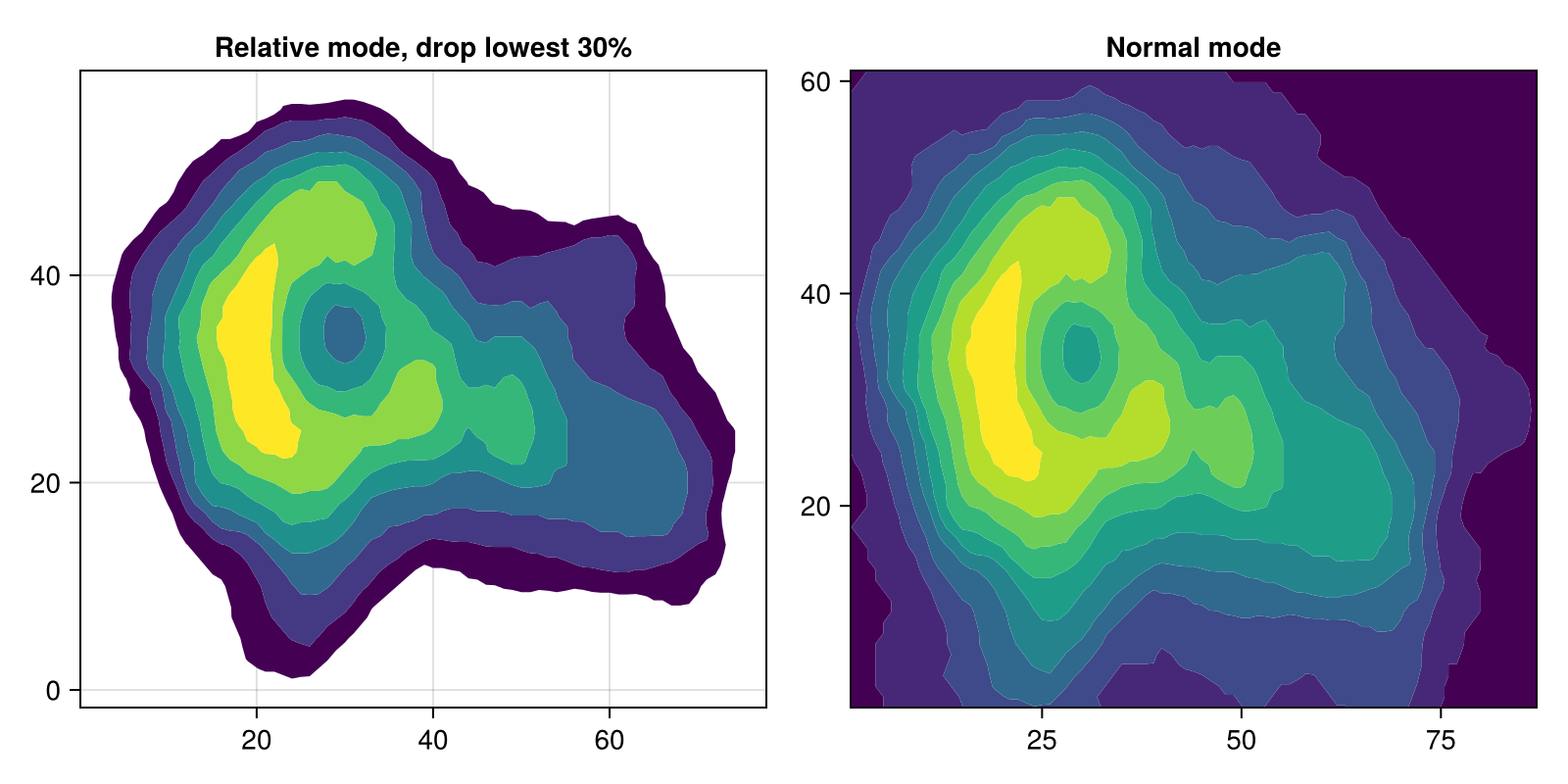

Curvilinear grids

contourf also supports curvilinear grids, where x and y are both matrices of the same size as z. This is similar to the input that surface accepts.

Let's warp a regular grid of x and y by some nonlinear function, and plot its contours:

using CairoMakie
x = -10:10
y = -10:10
# The curvilinear grid:
xs = [x + 0.01y^3 for x in x, y in y]
ys = [y + 10cos(x/40) for x in x, y in y]
# Now, for simplicity, we calculate the `zs` values to be
# the radius from the center of the grid (0, 10).
zs = sqrt.(xs .^ 2 .+ (ys .- 10) .^ 2)
# We can use Makie's tick finders to get some nice looking contour levels:
levels = Makie.get_tickvalues(Makie.LinearTicks(7), extrema(zs)...)
# and now, we plot!
f = Figure()
ax1 = Axis(f[1, 1])
ctrf1 = contourf!(ax1, x, y, zs; levels = levels)
ax2 = Axis(f[1, 2])
ctrf2 = contourf!(ax2, xs, ys, zs; levels = levels)
f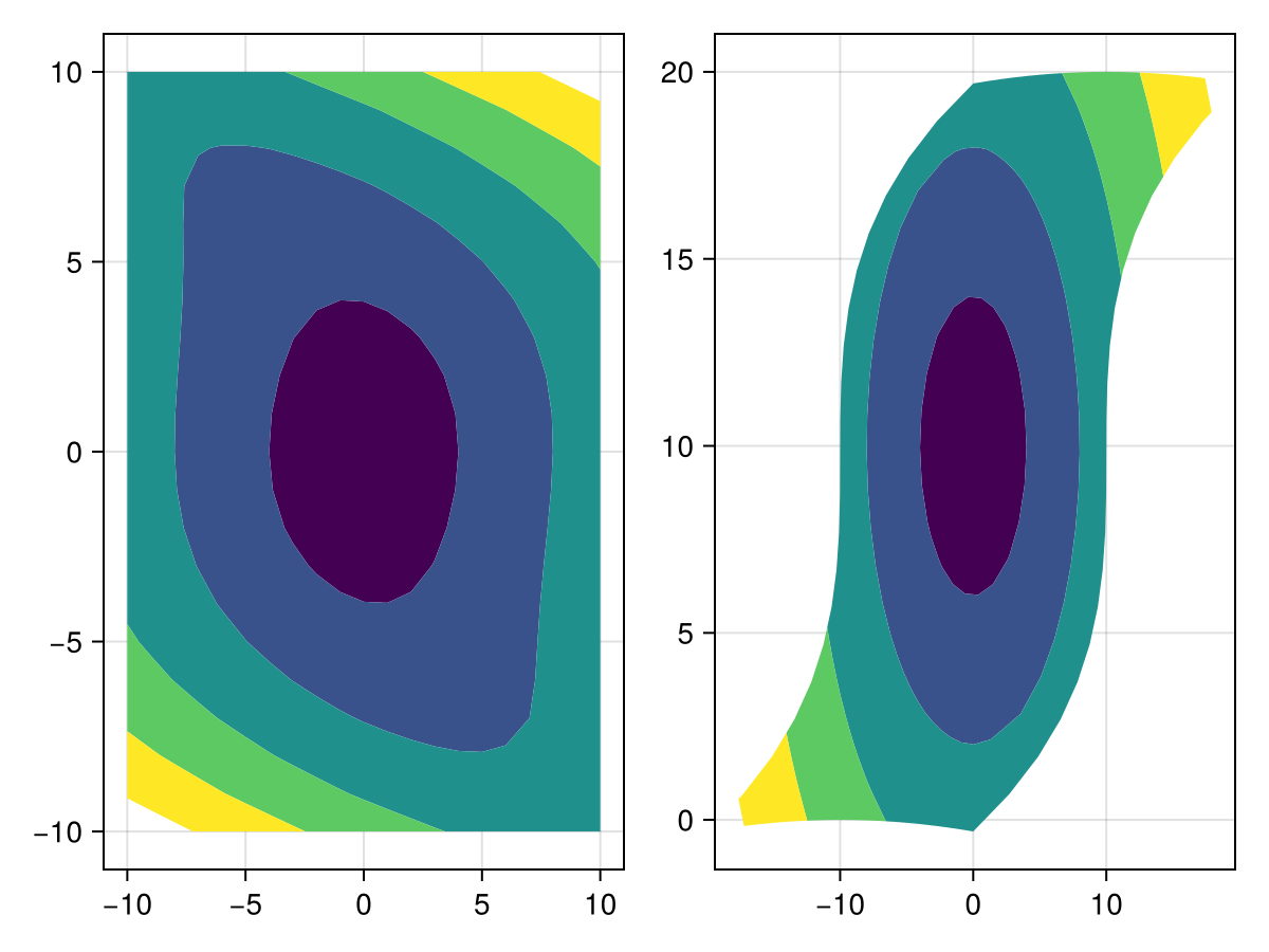

Attributes

clip_planes

Defaults to automatic

Clip planes offer a way to do clipping in 3D space. You can set a Vector of up to 8 Plane3f planes here, behind which plots will be clipped (i.e. become invisible). By default clip planes are inherited from the parent plot or scene. You can remove parent clip_planes by passing Plane3f[].

colormap

Defaults to @inherit colormap

No docs available.

colorscale

Defaults to identity

No docs available.

depth_shift

Defaults to 0.0

Adjusts the depth value of a plot after all other transformations, i.e. in clip space, where -1 <= depth <= 1. This only applies to GLMakie and WGLMakie and can be used to adjust render order (like a tunable overdraw).

extendhigh

Defaults to nothing

In :normal mode, if you want to show a band from the high edge to Inf, set extendhigh to :auto to give the extension the same color as the last level, or specify a color directly (default nothing means no extended band).

extendlow

Defaults to nothing

In :normal mode, if you want to show a band from -Inf to the low edge, set extendlow to :auto to give the extension the same color as the first level, or specify a color directly (default nothing means no extended band).

fxaa

Defaults to true

Adjusts whether the plot is rendered with fxaa (anti-aliasing, GLMakie only).

inspectable

Defaults to @inherit inspectable

Sets whether this plot should be seen by DataInspector. The default depends on the theme of the parent scene.

inspector_clear

Defaults to automatic

Sets a callback function (inspector, plot) -> ... for cleaning up custom indicators in DataInspector.

inspector_hover

Defaults to automatic

Sets a callback function (inspector, plot, index) -> ... which replaces the default show_data methods.

inspector_label

Defaults to automatic

Sets a callback function (plot, index, position) -> string which replaces the default label generated by DataInspector.

levels

Defaults to 10

Can be either

• an Int that produces n equally wide levels or bands

• an AbstractVector{<:Real} that lists n consecutive edges from low to high, which result in n-1 levels or bands

If levels is an Int, the contourf plot will be rectangular as all zs values will be covered edge to edge. This is why Axis defaults to tight limits for such contourf plots. If you specify levels as an AbstractVector{<:Real}, however, note that the axis limits include the default margins because the contourf plot can have an irregular shape. You can use tightlimits!(ax) to tighten the limits similar to the Int behavior.

mode

Defaults to :normal

Determines how the levels attribute is interpreted, either :normal or :relative. In :normal mode, the levels correspond directly to the z values. In :relative mode, you specify edges by the fraction between minimum and maximum value of zs. This can be used for example to draw bands for the upper 90% while excluding the lower 10% with levels = 0.1:0.1:1.0, mode = :relative.

model

Defaults to automatic

Sets a model matrix for the plot. This overrides adjustments made with translate!, rotate! and scale!.

nan_color

Defaults to :transparent

No docs available.

overdraw

Defaults to false

Controls if the plot will draw over other plots. This specifically means ignoring depth checks in GL backends

space

Defaults to :data

Sets the transformation space for box encompassing the plot. See Makie.spaces() for possible inputs.

ssao

Defaults to false

Adjusts whether the plot is rendered with ssao (screen space ambient occlusion). Note that this only makes sense in 3D plots and is only applicable with fxaa = true.

transformation

Defaults to :automatic

No docs available.

transparency

Defaults to false

Adjusts how the plot deals with transparency. In GLMakie transparency = true results in using Order Independent Transparency.

visible

Defaults to true

Controls whether the plot will be rendered or not.